第 4 章 参数化程序Chapter 4 Parameterized programs
神经网络可以被视为参数化程序:即带有可学习参数的程序。在本章中,我们首先回顾如何用数学方式表示程序。随后,我们回顾若干关键的神经网络架构与组件。Neural networks can be thought of as parameterized programs: programs with learnable parameters. In this chapter, we begin by reviewing how to represent programs mathematically. We then review several key neural network architectures and components.
4.1 表示计算机程序4.1 Representing computer programs
4.1.1 计算链Computation chains
首先,我们考虑这样一类简单程序:它对输入 依次施加一系列函数 。我们将这类程序称为计算链。例如,一张图像可以经历一系列变换,如裁剪、旋转、归一化等。在神经网络中,这些变换通常是参数化的,且参数是可学习的,由此得到 4.2 节介绍的前馈网络。函数序列的另一个例子是 for 循环,将在 5.8 节介绍。To begin with, we consider simple programs that apply a sequence of functions to an input . We call such programs computation chains. For example, an image may go through a sequence of transformations such as cropping, rotation, normalization, and so on. In neural networks, the transformations are typically parameterized, and the parameters are learned, leading to feedforward networks, presented in Section 4.2. Another example of a sequence of functions is a for loop, presented in Section 5.8.
形式上,计算链可以写为Formally, a computation chain can be written as
| (4.1) |
这里, 是输入, 是程序的中间状态, 是最终输出。当然, 的定义域(输入空间)必须与 的像(输出空间)相容。也就是说,应当有 。我们可以将计算链等价地写为Here, is the input, is an intermediate state of the program, and is the final output. Of course, the domain (input space) of must be compatible with the image (output space) of . That is, we should have . We can write a computation chain equivalently as
计算链可以用有向图表示,如图 4.1 所示。链中的边定义了一种全序。之所以是全序,是因为任意两个节点之间必然由一条路径相连。A computation chain can be represented by a directed graph, shown in Fig. 4.1. The edges in the chain define a total order. The order is total, since two nodes are necessarily linked to each other by a path.

4.1.2 有向无环图Directed acyclic graphs
在一般程序中,中间函数不仅可能依赖于前一个函数的输出,还可能依赖于若干不同函数的输出。这类依赖关系最好用图来表示。In generic programs, intermediate functions may depend, not only on the previous function output, but on the outputs of several different functions. Such dependencies are best expressed using graphs.
有向图 由一组顶点(或称节点) 以及一组刻画顶点之间有向依赖关系的边 共同定义。一条边 是一个有序的顶点对 与 。它也可记作 ,表示 依赖于 。为便于表示输入与输出,使用入半边 和出半边 会更为方便。A directed graph is defined by a set of vertices or nodes and a set of edges defining directed dependencies between vertices. An edge is an ordered pair of vertices and . It is also denoted , to indicate that depends on . For representing inputs and outputs, it will be convenient to use incoming half-edges and outgoing half-edges .
在图 中,顶点 的父节点是指向 的那些节点所构成的集合,记作 。顶点 的子节点则是 所指向的那些节点所构成的集合,即 。没有父节点的顶点称为根,没有子节点的顶点称为叶。In a graph , the parents of a vertex are the set of nodes pointing to , denoted . The children of a vertex are the set of nodes is pointing to, that is, . Vertices without parents are called roots and vertices without children are called leaves.
从 到 的路径由一个顶点序列 (可以为空)定义,且满足 。无环图是指这样的图:其中不存在顶点 ,使得存在从 到 的路径。有向无环图(DAG)则是指既是有向图、又是无环图的图。A path from to is defined by a sequence of vertices , potentially empty, such that . An acyclic graph is a graph such that there exists no vertex with a path from to . A directed acyclic graph (DAG) is a graph that is both directed and acyclic.
DAG 的边定义了顶点的一个偏序:若存在从 到 的路径,则记作 。该序是偏序,因为两个顶点不一定通过路径相互连接。尽管如此,我们可以定义一个称为拓扑序的全序:任意一种顺序,使得 当且仅当不存在从 到 的路径。The edges of a DAG define a partial order of the vertices, denoted if there exists a path from to . The order is partial, since two vertices may not necessarily be linked to each other by a path. Nevertheless, we can define a total order called a topological order: any order such that if and only if there is no path from to .
4.1.3 以 DAG 表示计算机程序Computer programs as DAGs
我们假定程序所定义的是一个数学上合法的函数(即纯函数):对相同的参数,程序返回相同的值,且不产生任何副作用。我们还假定程序会停机,即在有限步内终止。这样的程序由有限个中间函数与中间变量构成,因此函数与变量之间的依赖关系可以用有向无环图(DAG)来表示。不失一般性,我们作出如下简化假设:We assume that a program defines a mathematically valid function (a.k.a. pure function): the program should return identical values for identical arguments and should not have any side effects. We also assume that the program halts, i.e., that it terminates in a finite number of steps. As such a program is made of a finite number of intermediate functions and intermediate variables, the dependencies between functions and variables can be expressed using a directed acyclic graph (DAG). Without loss of generality, we make the following simplifying assumptions:
- 1.
程序只有一个输入 。There is a single input .
- 2.
程序只有一个输出 。There is a single output .
- 3.
程序中的每个中间函数 都只输出一个变量 。Each intermediate function in the program outputs a single variable .
我们将各节点依次编号为 。其中,节点 是根,对应输入 ;节点 是叶,对应最终的输出 。根据上述第三条假设,除 外,每个变量 都与一个函数 一一对应。因此,节点 表示输入 ,而节点 则既表示函数 ,又表示输出变量 。We number the nodes as . Node is the root, corresponding to the input . Node is the leaf, corresponding to the final output . Because of the third assumption above, apart from , each variable is in bijection with a function . Therefore, node represents the input , and nodes represent both a function and an output variable .
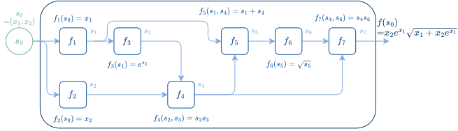
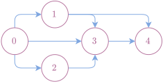
DAG 中的边表示依赖关系。节点 的父节点 (其中 )所表示的,正是函数 完成计算所需的变量 。换言之,父节点 表示在求解 之前必须先求值的函数 。图 4.3 给出了这一形式体系下的一个计算图示例。Edges in the DAG represent dependencies. The parents of node , where , indicate the variables that the function needs to perform its computation. Put differently, the parents indicate the functions that need to be evaluated, prior to evaluating . An example of a computation graph in our formalism is presented in Fig. 4.3.
执行程序Executing a program
要执行程序,必须保证按正确顺序对中间函数求值。为此,我们假定节点 已按拓扑序排列(若非如此,则需先进行拓扑排序)。于是,只要对 依次求值,便可执行程序To execute a program, we need to ensure that we evaluate the intermediate functions in the correct order. Therefore, we assume that the nodes are in a topological order (if this is not the case, we need to perform a topological sort first). We can then execute a program by evaluating for
注意, 既可视为以元素元组 为输入的单输入函数,也可视为以 为输入的多输入函数;这两种视角本质上是等价的。Note that we can either view as a single-input function of , which is a tuple of elements, or as a multi-input function of . The two views are essentially equivalent.
执行程序的过程总结于算法 1。The procedure for executing a program is summarized in Algorithm 1.
处理程序的多个输入或输出Dealing with multiple program inputs or outputs
当一个程序有多个输入时,我们总能把它们归入 ,作为 并带有 ,因为后续函数总能筛选出 中它们所需的元素。同样,如果一个中间函数 有多个输出,我们总能把它们归组为单个输出 并带有 ,因为后续函数可以筛选出 中它们所需的元素。When a program has multiple inputs, we can always group them into as with , since later functions can always filter out what elements of they need. Likewise, if an intermediate function has multiple outputs, we can always group them as a single output with , since later functions can filter out the elements of that they need.
另一种表示方式:二部图Alternative representation: bipartite graphs
在我们的形式体系中,由于函数 始终只有一个输出 ,节点 便可看作同时表示变量 与函数 。另一种做法如图 4.4 所示:将变量与函数表示为彼此分离的节点,即采用二部图。这种形式体系与概率建模中使用的因子图 [71, 121] 相近,只是其边为有向边。该形式体系的一个优点是能让函数显式地拥有多个输出。为简明起见,本书仍采用前一种形式体系。In our formalism, because a function always has a single output , a node can be seen as representing both the variable and the function . Alternatively, as shown in Fig. 4.4, we can represent variables and functions as separate nodes, that is, using a bipartite graph. This formalism is akin to factor graphs [71, 121] used in probabilistic modeling, but with directed edges. One advantage of this formalism is that it allows functions to explicitly have multiple outputs. We focus on our formalism for simplicity.


4.1.4 算术电路Arithmetic circuits
算术电路是计算图最简单的例子之一,源出计算复杂性理论。形式上,域 (例如实数集 )上的算术电路是一个有向无环图(DAG),其根节点为 的元素,其函数 或为 ,或为 。后者通常称为门。与一般计算图的情形不同,由于每个 或为 ,或为 ,因此必须允许图具有多个根节点。根节点既可以是变量,也可以是常数,且都应属于 。Arithmetic circuits are one of the simplest examples of computation graph, originating from computational complexity theory. Formally, an arithmetic circuit over a field , such as the reals , is a directed acyclic graph (DAG) whose root nodes are elements of and whose functions are either or . The latter are often called gates. Contrary to the general computation graph case, because each is either or , it is important to allow the graph to have several root nodes. Root nodes can be either variables or constants, and should belong to .
算术电路可用于计算多项式。同一个多项式可能有多个算术电路来表示。于是便产生一个重要问题:如何为计算给定多项式找到最高效的算术电路。为比较表示同一多项式的不同算术电路,一个直观的复杂度概念是电路规模,其定义如下。Arithmetic circuits can be used to compute polynomials. There are potentially multiple arithmetic circuits for representing a given polynomial. One important question is then to find the most efficient arithmetic circuit for computing a given polynomial. To compare arithmetic circuits representing the same polynomial, an intuitive notion of complexity is the circuit size, as defined below.
定义 4.1.1(电路规模与多项式规模)。Definition 4.1.1 (Circuit and polynomial sizes).
关于算术电路的更多内容,读者可参阅 [44] 的专著。For more information on arithmetic circuits, we refer the reader to the monograph of [44].
4.2 前馈网络4.2 Feedforward networks
前馈网络可视为由参数化函数 构成的计算链,A feedforward network can be seen as a computation chain with parameterized functions ,
其中给定输入 与可学习参数 。每个函数 称为一层,每个 可视为输入 的中间表示。 的维数称为第 层的宽度(或隐藏单元数)。前馈网络定义了从 到 的函数 ,其中 。for a given input and learnable parameters . Each function is called a layer and each can be seen as an intermediate representation of the input . The dimensionality of is known as the width (or number of hidden units) of layer . A feedforward network defines a function from to , where .
给定这样一个参数化程序,我们便可调整 以拟合某些数据,从而学习其中的参数。例如,给定由 对组成的数据集,我们可以关于 最小化在数据上平均的平方损失 。要最小化这样的损失,就需要获取其关于 的梯度。Given such a parameterized program, we can learn the parameters by adjusting to fit some data. For instance, given a dataset of pairs, we may minimize the squared loss on average over the data, w.r.t. . The minimization of such a loss requires accessing its gradients with respect to .
4.3 多层感知机4.3 Multilayer perceptrons
4.3.1 组合仿射层与激活函数Combining affine layers and activations
上一节没有说明如何参数化前馈网络。一种典型的参数化方式称为多层感知机(MLP),它采用如下形式的全连接(又称稠密)层:In the previous section, we did not specify how to parametrize the feedforward network. A typical parametrization, called the multilayer perceptron (MLP), uses fully-connected (also called dense) layers of the form
其中我们定义了元组 ,并假定 与 分别是尺寸适当的矩阵和向量。该层还可进一步分解为两个函数。函数 称为仿射层;函数 是一个无参数的非线性函数,通常称为激活函数(见 4.4 节)。值 通常称为预激活值,值 称为激活值。where we defined the tuple and where we assumed that and are a matrix and a vector of appropriate size. We can further decompose the layer into two functions. The function is called an affine layer. The function is a parameter-free nonlinearity, often called an activation function (see Section 4.4). The value is often called the pre-activation value and the value is the activation value.
更一般地,我们可以用关于 的任意参数化线性函数替代矩阵—向量乘积 。例如,卷积层将输入 与若干滤波器 的卷积视为一个线性映射。More generally, we may replace the matrix-vector product by any parametrized linear function of . For example, convolutional layers use the convolution of an input with some filters , seen as a linear map.
注 4.3.1(处理多个输入)。Remark 4.3.1 (Dealing with multiple inputs).
4.3.2 与广义线性模型的联系Link with generalized linear models
当深度为 (即只有一层)时,MLP 的输出为When the depth is (only one layer), the output of an MLP is
这称为广义线性模型(GLM),见 3.4 节。因此,MLP 将 GLM 作为特例包含在内。特别地,当 取 softargmax(见 4.4 节)时,我们便得到(多分类)logistic 回归。对于一般的深度 ,MLP 的输出为This is called a generalized linear model (GLM); see Section 3.4. Therefore, MLPs include GLMs as a special case. In particular, when is the softargmax (see Section 4.4), we obtain (multiclass) logistic regression. For general depth , the output of an MLP is
这可以看作是在输入 的学习表示 之上应用一个 GLM。这正是 MLP 的主要吸引力所在:它同时学习特征表示与输出模型!后文将会看到,MLP 也可以作为子组件用于其他架构。This can be seen as a GLM on top of learned representation of the input . This is the main appeal of MLPs: they learn the feature representation and the output model at the same time! We will see that MLPs can also be used as subcomponents in other architectures.
4.4 激活函数4.4 Activation functions
正如 4.3 节所述,前馈网络通常会在每一层使用激活函数 。本节介绍从标量到标量或从向量到标量的各种非线性函数,还会介绍可用作此类激活函数的概率映射。As we saw in Section 4.3, feedforward networks typically use an activation function at each layer. In this section, we present various nonlinearities from scalar to scalar or from vector to scalar. We also present probability mappings that can be used as such activations.
4.4.1 ReLU 与 softplusReLU and softplus
许多激活函数是标量到标量的函数,但也可以按逐元素方式应用于向量。ReLU(修正线性单元)是一种常用的非线性函数,定义为输入的非负部分Many activations are scalar-to-scalar functions, but they can also be applied to vectors in an element-wise fashion. The ReLU (rectified linear unit) is a popular nonlinearity defined as the non-negative part of its input
它是分段线性函数,在 处有一个折角。采用 ReLU 激活函数的多层感知机称为整流神经网络,其各层具有如下形式:It is a piecewise linear function and includes a kink at . A multilayer perceptron with ReLU activations is called a rectifier neural network. The layers take the form
其中 ReLU 按逐元素方式应用。ReLU 可替换为一种光滑近似(即不含折角),称为 softpluswhere the ReLU is applied element-wise. The ReLU can be replaced with a smooth approximation (i.e., without kinks), called the softplus
与 ReLU 不同,它始终严格为正。ReLU 还可有其他平滑变体,见 13.4 节。Unlike the ReLU, it is always strictly positive. Other smoothed variants of the ReLU are possible, see Section 13.4.
4.4.2 最大池化与 log-sum-expMax pooling and log-sum-exp
许多激活函数是向量到标量的函数:它们把向量归约为一个标量值。该标量值可视为一种统计量,用以“概括”该向量。Many activations are vector-to-scalar functions: they reduce vectors to a scalar value. This scalar value can be seen as a statistic, “summarizing” the vector.
最大池化Max pooling
向量到标量归约的一个例子是最大值,亦称最大池化。给定向量 ,其定义为An example of vector-to-scalar reduction is the maximum value, also known as max pooling. Given a vector , it is defined as
将 log-sum-exp 视为软最大值Log-sum-exp as a soft maximum
向量到标量归约的另一个例子是 log-sum-exp,Another example of vector-to-scalar reduction is the log-sum-exp,
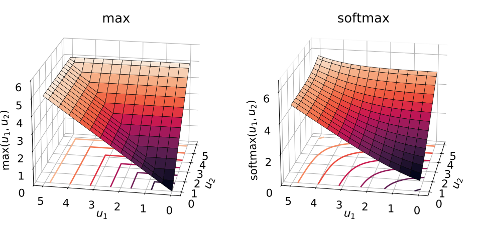
如图 4.5 所示,它已知具有软最大值的行为。log-sum-exp 可视为 softplus 的推广,因为对所有 都有As illustrated in Fig. 4.5, it is known to behave like a soft maximum. The log-sum-exp can be seen as a generalization of the softplus, as we have for all
log-sum-exp 的一种数值稳定实现如下:A numerically stable implementation of the log-sum-exp is given by
其中 。where .
更一般地,我们可以引入温度参数 More generally, we can introduce a temperature parameter
可以证明,对所有 ,It can be shown that for all ,
因此,当 时,。软最大值也可有其他定义,见 13.5 节。Therefore, as . Other definitions of soft maximum are possible; see Section 13.5.
将 log-sum-exp 视为对数域求和Log-sum-exp as a log-domain sum
除了用作软最大值,log-sum-exp 还常出现于对数域中的求和计算。事实上,假设要计算 ,其中 。若定义 与 ,则有Besides its use as a soft maximum, the log-sum-exp often arises for computing sums in the log domain. Indeed, suppose we want to compute , where . If we define and , we then have
换一种写法,我们得到恒等式Written differently, we have the identity
因此,可将 log-sum-exp 视为乘积恒等式的求和对应形式We can therefore see the log-sum-exp as the sum counterpart of the identity for products
例如,我们在 10.7.1 节中利用 log-sum-exp 在对数域中执行前向—后向算法。As an example, we use the log-sum-exp to perform the forward-backward algorithm in the log-domain in Section 10.7.1.
4.4.3 S 形函数:二值阶跃函数与 logistic 函数Sigmoids: binary step and logistic functions
我们常常希望把实数值映射到 中的某个数,用以表示某一事件的概率。为此,通常使用 S 形函数。S 形函数是曲线呈特征性“S”形的函数。这类函数是标量到标量的概率映射:用于把实数值压缩到 。Oftentimes, we want to map a real value to a number in , that can represent the probability of an event. For that purpose, we generally use sigmoids. A sigmoid is a function with a characteristic “S”-shaped curve. These functions are scalar-to-scalar probability mappings: they are used to squash real values to .
二值阶跃函数Binary step function
一个例子是二值阶跃函数,又称 Heaviside 阶跃函数,An example is the binary step function, also known as Heaviside step function,
它是从 到 的映射。遗憾的是,它并不连续:其图像在 处发生跳跃。此外,由于该函数在其余各点均为常数,因而在这些点处导数为零,这使其难以作为以反向传播训练的神经网络的一部分使用。It is a mapping from to . Unfortunately, it has a discontinuity: a jump in its graph at . Moreover, because the function is constant at all other points, it has zero derivative at these points, which makes it difficult to use as part of a neural network trained with backpropagation.
logistic 函数Logistic function
一种更好的 S 形函数是 logistic 函数,它是从 到 的映射,定义为A better sigmoid is the logistic function, which is a mapping from to and is defined as
它将 映射到 ,将 映射到 ,并满足 。因此,它可以看作是从实数值到概率值的映射。logistic 函数可以看作是不连续的二值阶跃函数 的可微近似。可以证明,logistic 函数是 softplus 的导数,即对所有 It maps to , to and it satisfies . It can therefore be seen as mapping from real values to probability values. The logistic can be seen as a differentiable approximation to the discontinuous binary step function . The logistic function can be shown to be the derivative of softplus, i.e., for all
logistic 函数的两个重要性质是:对所有 Two important properties of the logistic function are that for all
以及and
也可以采用其他 S 形函数;参见 13.6 节。Other sigmoids are possible; see Section 13.6.
4.4.4 概率映射:argmax 与 softargmaxProbability mappings: argmax and softargmax
将实向量变换为概率向量往往很有用。这是一个从 到概率单纯形的映射,定义为It is often useful to transform a real vector into a vector of probabilities. This is a mapping from to the probability simplex, defined by
这类向量到向量的概率映射有两个例子:argmax 与 softargmax。Two examples of such vector-to-vector probability mappings are the argmax and the softargmax.
ArgmaxArgmax
argmax 算子定义为The argmax operator is defined by
其中 表示整数 的 one-hot 编码,即where denotes the one-hot encoding of an integer , that is,
该映射把全部概率质量放在单个坐标上(若有并列,则任意选取一个坐标)。遗憾的是,该映射是不连续函数。This mapping puts all the probability mass onto a single coordinate (in case of ties, we pick a single coordinate arbitrarily). Unfortunately, this mapping is a discontinuous function.
SoftargmaxSoftargmax
作为一种处处可微的松弛,我们可以使用由下式定义的 softargmaxAs a differentiable everywhere relaxation, we can use the softargmax defined by
该算子在文献中通常称为 softmax,但这是一个误称:该算子实际上定义的是 argmax 的可微松弛。softargmax 的输出属于概率单纯形 的相对内部,这意味着它永远无法到达单纯形的边界。若记 ,则这意味着 ;也就是说, 永远不可能恰好等于 或 。 是 log-sum-exp 的梯度,This operator is commonly known in the literature as softmax but this is a misnomer: this operator really defines a differentiable relaxation of the argmax. The output of the softargmax belongs to the relative interior of the probability simplex , meaning that it can never reach the borders of the simplex. If we denote , this means that , that is, can never be exactly or . The is the gradient of log-sum-exp,
可以看作 logistic 函数的推广,因为对所有 都有The can be seen as a generalization of the logistic function, as we have for all
注 4.4.1(softargmax 的自由度与可逆性)。Remark 4.4.1 (Degrees of freedom and invertibility of softargmax).
4.5 归一化层4.5 Normalization layers
神经网络中的中间状态(如激活值)常常会取到各种不同的值,这可能使梯度下降难以收敛。为解决这一问题,我们可以在网络的适当位置引入归一化层。本节介绍两种最常用的归一化层:批归一化与层归一化。Intermediate states in neural networks, such as activations, can often attain a wide range of different values, potentially making it difficult for gradient descent to converge. To remedy this issue, we can introduce normalization layers at suitable locations in the network. In this section, we present the two most popular ones: batch normalization and layer normalization.
4.5.1 批归一化Batch normalization
假设给定一批中间变量(如激活值或状态),其中 ,这些变量由某个函数作用于从训练集中抽取的 个样本得到(为清晰起见,省略对层索引 的依赖)。在批归一化 [99] 中,我们计算批内样本上的标准分数(又称 z 分数)来归一化这些值,Suppose we are given a batch of intermediate variables (such as activations or states) , where , obtained by applying some function to samples drawn from the training set (we omit the dependency on the layer index for clarity). In batch normalization [99], we normalize the values by calculating the standard score (a.k.a. z-score) across batch samples,
其中,均值 与标准差 是针对每个特征 在批内样本 上计算的。实践中,我们常给 加上一个小量 ,以避免除零或数值不稳定。此外,我们常按下式对数值重新缩放:Here, the means and the standard deviations are computed for each feature across samples in the batch. In practice, we often add a small value to to avoid division by zero or numerical instabilities. Moreover, we often rescale the values as
其中均值 与标准差 是可学习参数。where the means and standard deviations are learnable parameters.
批归一化的一个问题在于,推断时无法计算均值 与标准差 ,因为推断时不存在训练批次的概念(单个样本会使方差为 )。为解决这一问题,我们可以在训练过程中估计整个训练集上的均值 与标准差 ,通常采用滑动平均。因此,实用的批归一化实现需要维护 个均值与标准差统计量,以便在推断时使用。One issue with batch normalization is that the means and standard deviations cannot be computed at inference time, as there is no notion of training batch (a single sample would lead to a variance of ). To address this issue, we can estimate means and standard deviations across the whole training set during the course of training, usually using a running average. A practical batch normalization implementation therefore needs to maintain mean and standard deviation statistics, so as to be able to use them at inference time.
4.5.2 层归一化Layer normalization
作为替代方案,层归一化 [6] 改为对特征求和来标准化数值,As an alternative, in layer normalization [6], we instead standardize the values by summing across features,
这一次,均值 与标准差 是针对每个样本 在特征 上计算的(如前,我们常给 加上一个小量 )。与批归一化类似,我们常按下式对数值重新缩放:This time, the means and the standard deviations are computed for each sample across features (as before, we often add a small value to ). Similarly to batch normalization, we often rescale the values as
其中均值 与标准差 是可学习参数。与批归一化相比,层归一化的一个关键优势在于它在推断时是良定义的:它按样本逐一应用,不依赖训练批次的概念。因此,我们可以把层归一化视为一个函数,它对任意 (无论是否属于某个批次)都对应where the means and standard deviations are learnable parameters. A key advantage of layer normalization compared to batch normalization is that it is well defined at inference time, since it is applied on a per-sample basis and does not rely on the notion of a training batch. As a result, we can view layer normalization as a function that to any (regardless of whether it is part of a batch or not) associates
4.6 残差神经网络4.6 Residual neural networks
现在我们讨论另一种前馈网络参数化:残差神经网络。考虑一个具有 层 、…、、 的前馈网络。当然,只要 能够精确表示恒等函数,该前馈网络所能表示的函数集合就应当是 、…、 所能表示的函数集合的超集。换句话说,从理论上讲,深度不应损害前馈网络的表达能力。然而,每个 都能精确表示恒等函数这一假设在实践中未必成立。这意味着更深的网络有时会比更浅的网络更难训练,从而使准确率随深度增加而饱和或下降。We now discuss another feedforward network parametrization: residual neural networks. Consider a feedforward network with layers , …, , . Surely, as long as can exactly represent the identity function, the set of functions that this feedforward network can express should be a superset of the functions that , …, can express. In other words, depth should in theory not hurt the expressive power of feedforward networks. Unfortunately, the assumption that each can exactly represent the identity function may not hold in practice. This means that deeper networks can sometimes be more difficult to train than shallower ones, making the accuracy saturate or degrade as a function of depth.
残差神经网络 [91] 的核心思想是设计称为残差块的层 ,使其更容易表示恒等函数。形式上,一个残差块具有如下形式The key idea of residual neural networks [91] is to design layers , called residual blocks, that make it easier to represent the identity function. Formally, a residual block takes the form
函数 称为残差,因为它建模的是差值 。与 相加通常称为跳跃连接。只要能够容易地调整 使 成立, 就能自由地变为恒等函数。例如,若采用The function is called residual, since it models the difference . The addition with is often called a skip connection. As long as it is easy to adjust so that , can freely become the identity function. For instance, if we use
其中 ,则只需将 与 分别设为零矩阵和零向量即可。已知残差块可以缓解所谓的梯度消失问题。where , it suffices to set and to a zero matrix and vector. Residual blocks are known to remedy the so-called vanishing gradient problem.
许多论文和软件包会加入一个额外的激活函数,并改为将残差块定义为Many papers and software packages include an additional activation and instead define the residual block as
其中 通常取为 ReLU 激活函数。是否加入这个额外的激活函数本质上是一种建模选择。在实践中,残差块还可能包含批归一化和卷积层等额外操作。where is typically chosen to be the ReLU activation. Whether to include this additional activation or not is essentially a modelling choice. In practice, residual blocks may also include additional operations such as batch norm and convolutional layers.
4.7 循环神经网络4.7 Recurrent neural networks
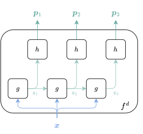
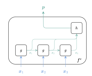
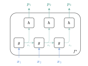
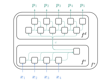
循环神经网络(RNN)是一类对向量序列进行运算的神经网络,这些序列可以作为输入、输出或两者兼有。其具体参数化取决于具体设定,但核心思想是维护一个状态向量,该向量由递归函数逐步更新,而该递归函数在各步之间共享参数。将这一递归展开,会得到一个有效的计算图,我们将在第 8 章看到这一点。我们区分图 4.7 所示的以下几种设定:Recurrent neural networks (RNNs) are a class of neural networks that operate on sequences of vectors, either as input, output or both. Their actual parametrization depends on the setup but the core idea is to maintain a state vector that is updated from step to step by a recursive function that uses shared parameters across steps. Unrolling this recursion defines a valid computational graph, as we will see in Chapter 8. We distinguish between the following setups illustrated in Fig. 4.7:
- •
向量到序列(一对多):Vector to sequence (one to many):
- •
序列到向量(多对一):Sequence to vector (many to one):
- •
序列到序列(多对多,对齐):Sequence to sequence (many to many, aligned):
- •
序列到序列(多对多,未对齐):Sequence to sequence (many to many, unaligned):
其中 表示长度。注意,为记号方便,我们对每种设定都使用相同数量的参数 ,当然实际情况未必如此。本节中,我们用记号 表示由 个向量构成的序列。where stands for length. Note that we use the same number of parameters for each setup for notational convenience, but this of course does not need to be the case. Throughout this section, we use the notation for a sequence of vectors.
4.7.1 向量到序列Vector to sequence
在此设定下,我们定义解码器函数 ,它从输入向量 和参数 映射到输出序列 。例如,这对于图像描述生成很有用,即从一张图像(像素向量)生成一个句子(词嵌入序列)。形式上,我们可以通过递归定义 In this setting, we define a decoder function from an input vector and parameters to an output sequence . This is for instance useful for image caption generation, where a sentence (a sequence of word embeddings) is generated from an image (a vector of pixels). Formally, we may define through the recursion
其中 。 的目标是在给定输入 和前一解码器状态 的情况下,更新当前解码器状态 。 的目标是在给定当前解码器状态 的情况下生成输出 。重要的是, 与 的参数在各步之间共享。通常, 与 使用单隐藏层 MLP 参数化。注意, 有多个输入;我们将在 4.3 节讨论如何处理这类情形。where . The goal of is to update the current decoder state given the input , and the previous decoder state . The goal of is to generate the output given the current decoder state . Importantly, the parameters of and are shared across steps. Typically, and are parametrized using one-hidden-layer MLPs. Note that has multiple inputs; we discuss how to deal with such cases in Section 4.3.
4.7.2 序列到向量Sequence to vector
在此设定下,我们定义编码器函数 ,它从输入序列 和参数 映射到输出向量 。例如,这对于序列分类(如情感分析)很有用。形式上,我们可以用递归定义 In this setting, we define an encoder function from an input sequence and parameters to an output vector . This is for instance useful for sequence classification, such as sentiment analysis. Formally, we may define using the recursion
其中 。 的目标与 类似,区别在于它更新编码器状态,且不将先前的预测作为输入。池化函数通常不带参数。其目标是将序列归约为一个向量。示例包括使用最后一个状态、状态的均值以及状态的按坐标最大值。where . The goal of is similar to , except that it updates encoder states and does not take previous predictions as input. The pooling function is typically parameter-less. Its goal is to reduce a sequence to a vector. Examples include using the last state, the average of states and the coordinate-wise maximum of states.
4.7.3 序列到序列(对齐)Sequence to sequence (aligned)
在此设定下,我们定义函数 :它从输入序列 与参数 出发,映射得到输出序列 ,并假定两者长度相同。一个应用示例是词性标注,其目标是为每个词 标注词性(名词、动词、形容词等)。形式上,我们可以将 定义为In this setting, we define a function from an input sequence and parameters to an output sequence , which we assume to be of the same length. An example of application is part-of-speech tagging, where the goal is to assign each word to a part-of-speech (noun, verb, adjective, etc). Formally, we may define as
其中 。函数 与 的含义与前述相同。where . The functions and are similar as before.
4.7.4 序列到序列(未对齐)Sequence to sequence (unaligned)
在此设定下,我们定义函数 :它从输入序列 与参数 出发,映射得到输出序列 ,而两者长度可以不同。一个应用示例是机器翻译,其中源语言与目标语言的句子未必等长。通常, 由以下两个步骤定义In this setting, we define a function from an input sequence and parameters to an output sequence , which potentially has a different length. An example of application is machine translation, where the sentences in the source and target languages do not necessarily have the same length. Typically, is defined as the following two steps
其中 ,并复用了先前定义的编码器 与解码器 。将两步合并,可得where , and where we reused the previously-defined encoder and decoder . Putting the two steps together, we obtain
这一架构恰如其分地被称为编码器—解码器架构。注意,我们把目标序列的长度记为 。然而在实践中,目标长度可能取决于输入,而且往往无法预先得知。为解决这一问题,通常会在词表(按本书记号,其大小为 )中额外加入一个“序列结束”(EOS)标记,从而在推断时便知道何时停止生成输出序列。不过,这种编码器—解码器架构有一个缺点:输入序列的全部信息都集中于上下文向量 之中,因此该向量可能成为瓶颈。This architecture is aptly named the encoder-decoder architecture. Note that we denoted the length of the target sequence as . However, in practice, the target length can be input dependent and is often not known ahead of time. To deal with this issue, the vocabulary (of size in our notation) is typically augmented with an “end of sequence” (EOS) token so that, at inference time, we know when to stop generating the output sequence. One disadvantage of this encoder-decoder architecture, however, is that all the information about the input sequence is contained in the context vector , which can therefore become a bottleneck.
4.8 transformer4.8 Transformers
transformer [199] 是近年来深度学习领域最成功的进展之一。本节将逐一剖析 transformer 的各个组件。Transformers [199] are one of the most successful recent developments in deep learning. In this section, we review Transformers, component by component.
4.8.1 注意力Attention
注意力层的目标是将输入序列 映射为维度相同的输出序列 。一个自然的思路是:以输入元素的线性组合来定义每个输出元素 ,The goal of an attention layer is to map a sequence of inputs to a sequence of outputs , of same dimension. A natural idea is to define each output element using a linear combination of the input elements,
我们通常采用凸组合:假定组合权重满足 。这样便保证了,在增大某一系数 时,必然要以减小另一系数 为代价,其中 。把 与 视为行向量并加以堆叠,我们便得到矩阵 和 。我们还可构造注意力矩阵 ,用以汇集元素 ;其中 表示按行随机的 矩阵之集。于是,注意力便可简洁地重写为We typically use a convex combination: we assume that the combination weights are such that . This ensures that increasing a coefficient is made at the expense of decreasing another coefficient , for . Let us form the matrices and by stacking and , seen as row vectors. Let us also form the attention matrix gathering the entries , where denotes the set of row-wise stochastic matrices. Then, we can rewrite attention succinctly as
参照 6.2 节,我们可以把注意力视为一种软字典查找。从这个视角看,矩阵 扮演字典值的角色,而注意力矩阵可定义为Following Section 6.2, we can view attention as a soft dictionary lookup. From this perspective, the matrix plays the role of dictionary values, and the attention matrix can be defined as
其中 与 分别扮演查询与字典键的角色。直观而言, 可看作一个相似度矩阵,包含查询与字典键之间的相似度。将上述各部分合在一起,我们便可把注意力定义为where and play the roles of queries and dictionary keys, respectively. Intuitively, can be seen as a similarity matrix containing the similarities between queries and dictionary keys. Putting everything together, we can define attention as
在掩码注意力中,我们额外引入一个掩码 ,In masked attention, we additionally incorporate a mask ,
其中 表示 Hadamard 乘积(逐元素乘积)。通过把相应的掩码元素 设为 ,该掩码可强制某些注意力权重 为零。例如,在仅解码器架构(4.8.8 节)中,该掩码将有助于为自回归模型定义因果注意力。where denotes the Hadamard product (element-wise multiplication). The mask can be used to force some attention weights to be zero, by setting the corresponding mask entry to . For instance, in decoder-only architectures (Section 4.8.8), the mask will prove useful to define causal attention for autoregressive models.
注 4.8.1(缩放注意力)。Remark 4.8.1 (Scaled attention).
4.8.2 自注意力Self-attention
假设给定一个特征向量序列 ,并将其汇集为矩阵 。为定义注意力权重 ,一个自然的想法是考虑 与 之间的相似度,以内积 来衡量。为确保 ,我们便可定义Suppose we are given a sequence of feature vectors , that we gather as a matrix . To define the attention weights , a natural idea is to consider the similarity between and , as measured by the inner product . To ensure that , we can then define
用矩阵记号,这可写成In matrix notation, this can be written
其中 按行逐一施加。矩阵 是与行向量 相关联的 Gram 矩阵。按上一节的记号,这相当于取 ,其中 。换言之,序列中的各元素彼此“关注”,这被称为自注意力。where is applied in a row-wise fashion. The matrix is the Gram matrix associated with the row vectors . In the notation of the previous section, this corresponds to using with . In other words, the elements of the sequence “pay attention” to each other. This is called self-attention.
前文所述的表述方式不含参数。为增强自注意力层的表达能力,[199] 提出改为将 投影,以此定义 、 与 :So far, the formulation we described is parameter-free. To give more expressive power to the self-attention layer, [199] proposed instead to define , and by projecting as
使用学习到的权重矩阵using the learned weight matrices
关键在于,权重矩阵的大小与序列长度 无关。因此,自注意力可以处理任意长度的序列。Importantly, the size of the weight matrices is independent of the length of the sequences. This allows self-attention to work with sequences of arbitrary length.
4.8.3 多头注意力Multi-head attention
为了捕捉多种注意力模式,[199] 发现定义 个注意力头会带来收益In order to be able to capture multiple patterns of attention, [199] found it beneficial to define attention heads
其中where
使用已学习的权重矩阵using the learned weight matrices
将 个注意力头拼接,记为Let us denote the concatenation of the attention heads by
随后,[199] 将多头注意力定义为[199] then define multi-head attention as
其中 为可学习矩阵。该过程总结于算法 2。为清晰起见,我们用 for 循环表述;而面向 GPU 的实现则改用单次矩阵乘法。where is a learned matrix. We summarize the procedure in Algorithm 2. We use a for loop for the sake of clarity; a GPU-friendly implementation would instead be based on a single matrix multiplication.
4.8.4 Transformer 层Transformer layer
为提高训练效率,可引入残差连接与第一层归一化(4.5.2 节),从而定义To improve training efficiency, we can introduce residual connections and a first layer normalization (Section 4.5.2), to define
为增强表达能力,Transformer 层进一步使用一个 MLP 与第二个层归一化,To improve expressiveness, a Transformer layer further uses an MLP and a second layer normalization,
中的下标意在强调:这两层各自使用独立的参数。此外,归一化按逐元素(逐 token)方式进行。MLP 块通常采用带激活函数 的单个隐藏层,例如 GELU(高斯误差线性单元),见算法 3。由于使用了残差连接,MLP 块的输入与输出维度必须相同。The subscripts in are used to emphasize that the two layers use their own parameters. In addition, normalization is applied in an element-wise (token-wise) fashion. The MLP block typically uses a single hidden layer with an activation function , such as a GELU (Gaussian error linear unit); see Algorithm 3. Because of the use of residual connections, the input and output dimensions of the MLP block must be the same.
注 4.8.2(后归一化与预归一化)。Remark 4.8.2 (Post-normalization vs. pre-normalization).
4.8.5 Transformer 块Transformer block
将 Transformer 层迭代 次(每次使用不同参数),即可定义深度为 的 Transformer 块。若隐去对参数的依赖,则可将带可选掩码 的 Transformer 视为一个函数,A Transformer layer can be iterated times (each time with different parameters) to define a Transformer block of depth . Keeping the dependency on parameters implicit, we can see a Transformer, with an optional mask , as a function
从 映射到 。Transformer 接收序列 ,并利用序列元素之间的相互依赖关系生成该序列的表示。该过程总结于算法 4。、 与 各块均以 为索引,以强调其参数在每次迭代中互不相同。from to . The Transformer takes a sequence and uses the inter-dependencies between sequence elements to produce a representation of that sequence. We summarize the procedure in Algorithm 4. The , and blocks are indexed by to emphasize that their parameters are different for each iteration.
参数数量与计算复杂度Number of parameters and computational complexity
Transformer 层可视为从 到 的函数。若要让标准多层感知机具有相同的函数签名,则需要 个参数,且其一次网络前向传播的时间复杂度同样为 。相比之下,一个 Transformer 层只有 个参数。其中,自注意力的复杂度为 ,最后的 MLP 层复杂度为 。The Transformer layer can be seen as a function from to . To offer the same function signature, a standard multi-layer perceptron would have needed parameters and a forward pass through the network would have had a time complexity of as well. In contrast, a Transformer layer has parameters. Self-attention has a complexity of and the final MLP layer has a complexity of .
4.8.6 token 编码Token encoding
文本可表示为由离散符号构成的序列 ,这些符号通常称为 token。此处每个 token (其中 为词表大小)可对应单词、子词,乃至单个字符,具体取决于分词方式。为得到连续向量序列 (其中 ),通常采用嵌入层。该层通过线性投影将 变换为 ,Text can be represented as a sequence of discrete symbols, often called tokens. Here, each token , where is the vocabulary size, can correspond to words, subwords, or even individual characters, depending on the tokenization procedure. To obtain a sequence of continuous vectors , where , it is common to use an embedding layer. This layer transforms into using the linear projection
其中 为 的 one-hot 编码, 为可学习的嵌入矩阵。列 可解释为 token 的连续表示。词表通常还包含特殊 token,如“BOS”(序列开始)、“EOS”(序列结束)与“PAD”(填充 token,用于保证序列长度为 )。where is the one-hot encoding of and is a learnable embedding matrix. The column can be interpreted as the continuous representation of token . Usually, the vocabulary includes special tokens such as “BOS” (beginning of sequence), “EOS” (end of sequence) and “PAD” (padding token, to ensure that the sequence is of length ).
4.8.7 位置编码Positional encoding
受其参数化方式影响,Transformer 对置换具有等变性:先置换输入序列再施加 Transformer,与先施加 Transformer 再置换输出序列,二者等价。形式上,对任意大小为 的置换矩阵 ,以及视为矩阵 的输入序列 ,均有Due to their parameterization, Transformers are equivariant with respect to permutations: permuting the input sequence and applying the Transformer is equivalent to applying the Transformer and permuting the output sequence. Formally, for any permutation matrix of size and input sequence seen as a matrix , we have
这意味着 Transformer 将有序序列视为多重集(多重集是对集合概念的修改,允许其中元素出现多个实例)。若要在 Transformer 中利用顺序信息,有若干可行途径 [60]:加入位置编码(绝对或相对)、修改注意力矩阵,或用 RNN 对输入序列作预处理。加入位置编码时,通常将表示位置 的向量 加到相应元素 之上,This means that Transformers treat an ordered sequence as a multi-set (a modification of the concept of a set that allows for multiple instances of its elements). To leverage order information in a Transformer, several approaches are possible [60]: adding positional encoding (either absolute or relative), modifying the attention matrix and pre-processing the input sequence with an RNN. To add positional encoding, one typically adds a vector representing the position to the corresponding element ,
理想的位置编码应当适用于任意序列长度。An ideal positional encoding should work with any sequence length.
可学习的位置编码Learned positional encoding
与 token 编码类似,定义位置编码的一个简便方法是使用嵌入层。每个位置 经由下式变换为位置向量 :Similarly to the token encoding, a simple way to define a positional encoding is to use an embedding layer. Each position is transformed into a position vector by
其中 是 的 one-hot 编码, 是可学习的嵌入矩阵。列 可解释为位置 的连续表示。where is the one-hot encoding of and is a learnable embedding matrix. The column can be interpreted as the continuous representation of position .
正弦位置编码Sinusoidal positional encoding
我们不必学习位置编码,也可以用启发式方式定义它。例如,[199] 提出了正弦位置编码 ,其定义为Instead of learning the positional encoding, we can define it in a heuristic manner. For instance, [199] proposed the sinusoidal positional encoding , defined by
其中where
并且其中 是常数,作者将其设为 。我们可以把所有取值汇总为一个位置编码矩阵 ,如图 4.8 所示。and where is a constant, set to by the authors. We can gather the values in a position encoding matrix , as depicted in Fig. 4.8.
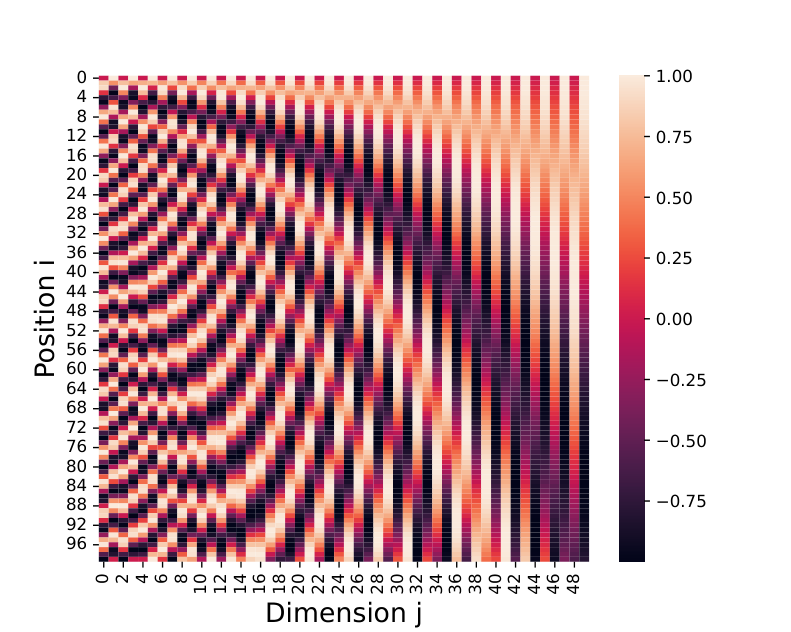
乍看之下,正弦位置编码或许显得有些神秘。为获得一些直观理解,可以将其与整数的离散二进制编码进行比较,On first sight, sinusoidal positional encoding may seem a bit mysterious. To gain some intuition, it is useful to compare it to a discrete binary encoding of integers,
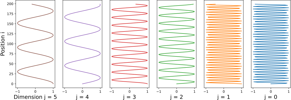
我们可以看到,从右向左移动时,比特在 与 之间的交替变得更加频繁。正弦位置编码实现了类似的行为,只不过它是连续的。实际上,每个坐标 都对应一条正弦波(当 为偶数时)或余弦波(当 为奇数时)。与 关联的波的波长或周期为 ,频率为 。由于 是关于 的递减函数,可以看到,当 较小时,波的振荡更为频繁。图 4.9 展示了这一行为。We see that the bits alternate more frequently between and as we go from right to left. The sinusoidal positional encoding achieves a similar behavior, but is continuous. Indeed, each coordinate is associated with a sine wave (when is even) or a cosine wave (when is odd). The wavelength or period of the wave associated with is and its frequency is . Since is a decreasing function of , we see that the waves oscillate more frequently when is small. This behavior is illustrated in Fig. 4.9.
将正弦波与余弦波堆叠起来,已被用于构造随机傅里叶特征 [165, 190]。这些方法使用随机频率的波,而正弦位置编码使用频率递增的波。因此,两者的主要区别在于波频率的选择方式。Stacking sine and cosine waves has been used for creating random Fourier features [165, 190]. These use waves of random frequencies, while sinusoidal positional encoding uses waves of increasing frequency. These approaches therefore mainly differ in the way we choose wave frequencies.
恢复相对位置信息Recovering relative positional information
正弦位置编码的一个重要性质是:对于任意偏移量 , 都可以表示为 的线性函数 [199, 214]。因此,模型应当能够轻松学会依据相对位置进行注意力计算。事实上,利用关于角和的三角恒等式An important property of the sinusoidal positional encoding is that can be represented as a linear function of , for any offset [199, 214]. The model should therefore be able to easily learn to attend by relative positions. Indeed, using the trigonometric identities for angle sums
对于偶数 ,我们有we have for even
因此,通过施加一个旋转矩阵, 可以被线性投影为 。这使得 Transformer 能够轻松学会依据相对位置进行注意力计算。Therefore, can be linearly projected to , by applying a rotation matrix. This allows a Transformer to easily learn to attend by relative positions.
旋转位置编码(RoPE)Rotary positional encoding (RoPE)
在自注意力中考虑绝对位置信息的另一种流行方法是 RoPE [189],它代表旋转位置编码(rotary positional encoding)。为简单起见,我们以单个注意力头和 为例简要说明其思想。假设我们有一个已经用 token 编码编好的序列 。随后,我们将查询向量和键向量定义为Another popular approach for taking into account absolute positional information in self-attention is RoPE [189], which stands for rotary positional encoding. For simplicity, we briefly explain the idea with a single attention head and . Suppose we have a sequence already encoded with token encoding. We then define the query and key vectors as
其中 是旋转矩阵。其核心直觉是,我们将这个 维向量旋转一个角度,该角度是位置 的倍数。与可学习位置编码和正弦位置编码不同,权重矩阵 和 是在施加 RoPE 之前应用的,而不是之后。where is a rotation matrix. The main intuition is that we are rotating the -dimensional vector by an angle which is a multiple of the position . In contrast to the learned and sinusoidal positional encodings, the weight matrices and are applied before applying RoPE, not after.
当 时, 定义为旋转矩阵When , is defined as the rotation matrix
其中角度为 、位置为 。利用欧拉公式for some angle and position . Using Euler’s formula
我们注意到,对于 和 , 等价于对于 和 的 。RoPE 公式的详细推导参见 [189]。we note that for and is equivalent to for and . See [189] for a detailed derivation of RoPE’s formula.
当 时,假设 为偶数, 定义为When , assuming is even, is defined as
其中 。在实践中,我们从不把 具体化为矩阵,因为它会非常稀疏;相反,我们将其视为作用在任意向量 上的线性映射,where . In practice, we never materialize as a matrix, since it would be very sparse, but rather view it as a linear map applied to an arbitrary vector ,
一旦计算出 和 ,我们就可以像往常一样使用 。对于多头注意力,我们只需对每个注意力头应用相同的方法。Once we computed and , we can use as usual. For multi-head attention, we simply apply the same approach for each attention head.
正如 [189] 所分析的,RoPE 具备若干有价值的性质。特别是,它关于序列长度 是灵活的;尽管它是一种绝对编码,却也能捕捉 token 之间的相对距离。因此,它兼具绝对位置编码与相对位置编码的优点。As analyzed by [189], RoPE satisfies several valuable properties. In particular, it is flexible w.r.t. the sequence length and despite being an absolute encoding, it manages to also capture relative distance between tokens. It therefore has the merits of both absolute and relative positional encodings.
4.8.8 仅解码器架构Decoder-only architectures
定义语言模型Defining a language model
Transformer 最初是为机器翻译构建编码器—解码器架构而提出的 [199]。然而,在语言建模的语境下,Transformer 如今通常采用仅解码器的自回归架构。假设给定一个离散符号序列 (若序列元素少于 个,可以使用填充符号)。(无条件的)语言模型的目标是构造一个产生联合概率的函数,Transformers were originally developed to create encoder-decoder architectures for machine translation [199]. However, in the context of language modelling, Transformers are now routinely used for decoder-only autoregressive architectures. Suppose we are given a sequence of discrete symbols (if a sequence has less than elements, we can use padding symbols). The goal of (unconditional) language models is to create a function producing the joint probability,
利用概率的链式法则(10.1 节),不失一般性,我们可以将其写成Using the chain rule of probability (Section 10.1), without loss of generality, we can write
如果最大长度 非常大,更实用的做法是只考虑大小为 的上下文窗口,If the maximum length is very large, it is more practical to only consider a context window of size ,
这相当于定义一个高阶马尔可夫链(10.4.3 节)。采用这种方法,构建语言模型便归结为定义一个函数This amounts to defining a higher-order Markov chain (Section 10.4.3). Using this approach, creating a language model then boils down to defining a function
假设离散符号序列 已通过 token 编码(4.8.6 节)和位置编码(4.8.7 节)映射为连续向量序列 。使用因果 Transformer 块,我们可以获得当前上下文的表示,Let us assume that the sequence of discrete symbols has been mapped to a sequence of continuous vectors using token encoding (Section 4.8.6) and positional encoding (Section 4.8.7). Using a causal Transformer block, we can obtain a representation of the current context,
为确保 Transformer 仅依赖过去的 token 来预测当前 token,掩码矩阵 被设为大小为 的矩阵,其下三角部分元素设为 ,上三角部分元素设为 。为将其归约为 中的 logit,我们通常使用上下文的最后一个元素 并应用一个线性模型,得到To ensure that the Transformer only relies on past tokens to predict the current token, the mask matrix is set to a matrix of size , with the elements of the lower part set to , and the elements of the upper part set to . To reduce this to logits in , we usually use the last element of the context and apply a linear model, to obtain
其中 是一个可学习的“解嵌入”矩阵。为得到有效的概率分布,我们对 logit 应用 soft-argmax,where is a learned “disembedding” matrix. To obtain a valid probability distribution, we apply a soft-argmax on the logits ,
最后,我们现在可以定义Finally, we can now define
注 4.8.3(权重绑定)。Remark 4.8.3 (Weight tying).
训练Training
我们将 Transformer 的参数(多头注意力、MLP、层归一化)汇总记为 。于是,上下文窗口大小为 的仅解码器 Transformer 定义了一个参数化概率分布Let us gather the Transformer parameters (multi-head attention, MLP, layer norm) as . The decoder-only Transformer with a context window of size then defines a parametric probability distribution
给定一个序列语料 ,我们通常通过最大化对数似然来求参数 ,Given a corpus of sequences , we usually seek the parameters by maximizing the log-likelihood,
这相当于以逐 token 的方式使用 logistic(交叉熵)损失。重要的是,用于预测下一个 token 的上下文 始终来自数据,而非模型生成的 token。这被称为教师强制,它使 Transformer 的训练高度可并行化。该目标通常使用随机梯度算法近似求解。为最大化 GPU 利用率,通常将长度可变的序列打包在一起以组成批次。This amounts to using a logistic (cross-entropy) loss in a token-wise fashion. Importantly, the context used to predict the next token always comes from the data, not from the tokens generated by the model. This is called teacher forcing and makes Transformer training highly parallelizable. The objective is usually solved approximately using stochastic gradient algorithms. To maximize GPU utilization, sequences of variable lengths are usually packed together in order to form batches.
采样Sampling
上下文窗口大小为 的仅解码器 Transformer,可视为构成一条高阶马尔可夫链,而高阶马尔可夫链是贝叶斯网络的一种特例。因此,要从该模型中生成序列,我们可以采用祖先采样(10.5.3 节),A decoder-only Transformer with a context window of size can be seen as forming a higher-order Markov chain, which is a special case of Bayesian network. To generate a sequence from the model, we can therefore use ancestral sampling (Section 10.5.3),
其中 表示序列开始(BOS)token。当生成序列结束(EOS)token,或达到最大长度时,采样即停止。所生成的序列是独立同分布的。where denotes the beginning-of-sequence (BOS) token. The sampling stops when the end-of-sequence (EOS) token is generated or when a maximum length is reached. The generated sequences are i.i.d. .
由于采样一次只产生一个 token,因此这一过程高度串行。Transformer 块按如下方式依次调用:Because sampling happens one token at a time, it is highly sequential. The Transformer block is called sequentially as
| … | |
为避免反复进行相同的计算,在假定使用因果掩码的前提下,多头注意力(4.8.3 节)中用到的过去的键矩阵与值矩阵通常存入所谓的 KV 缓存。To avoid repeating the same computations again and again, assuming that a causal mask is used, the past key and value matrices used in multi-head attention (Section 4.8.3) are usually stored in the so-called KV cache.
4.8.9 仅编码器架构Encoder-only architectures
仅编码器 Transformer 可用于学习序列的表示。最突出的例子是 BERT [56],其全称为来自 Transformer 的双向编码器表示。BERT 使用不带因果掩码的算法 4(缩写中的“双向”即由此而来)。离散序列元素经 token 编码、位置编码以及可能的段编码转换为向量。出于下文即将说明的原因,每个序列的第一个 token 始终是一个特殊的分类 token [CLS]。训练分为两个阶段:预训练与微调。Encoder-only Transformers can be used for learning to represent sequences. The most prominent example is BERT [56], which stands for bidirectional encoder representations from transformers. BERT uses Algorithm 4 without causal mask (hence “bidirectional” in the acronym). Discrete sequence elements are transformed to vectors using token encoding, positional encoding and potentially segment encoding. For reasons that will become clear below, the first token of every sequence is always a special classification token [CLS]. Training is broken down into two phases: pretraining and finetuning.
预训练Pretraining
由于预训练在无标签语料上进行,因此需要合成预测任务。Since pre-training is performed on an unlabeled corpus, it is necessary to synthetically generate prediction tasks.
在掩码预测中,按一定比例(通常为 15%)对输入 token 随机施加掩码。随后训练模型,依据未被掩码的 token 所提供的上下文,预测被掩码 token 的原始词表 ID。这迫使模型学习一种丰富的、双向的语言表示。掩码策略包括:In masked prediction, a percentage (typically 15%) of the input tokens are randomly masked. The model is then trained to predict the original vocabulary ID of the masked tokens, given the context provided by the unmasked tokens. This forces the model to learn a rich, bidirectional representation of the language. The masking strategy involves:
- •
80% 的情况下,将选中的 token 替换为 [MASK];80% of the time, replacing the chosen token with [MASK],
- •
10% 的情况下,将选中的 token 替换为词表中的随机 token;10% of the time, replacing the chosen token with a random token from the vocabulary,
- •
10% 的情况下,保持选中的 token 不变。10% of the time, keeping the chosen token unchanged.
在下一句预测中,模型被训练以理解两个句子之间的关系。对每个训练样本,BERT 会收到两个句子 和 。50% 的情况下,B 是原始文档中紧接 A 之后的真实下一句(标记为 IsNext);另外 50% 的情况下, 是语料中的随机句子(标记为 NotNext)。输入序列开头会添加一个特殊的 [CLS] token,其最终隐藏状态用于预测句子 是否紧接句子 A。[SEP] token 用于分隔这两个句子。In next sentence prediction, the model is trained to understand the relationship between two sentences. For each training example, BERT is given two sentences, and . 50% of the time, B is the actual next sentence that follows A in the original document (labeled IsNext). The other 50% of the time, is a random sentence from the corpus (labeled NotNext). A special [CLS] token is prepended to the input sequence, and its final hidden state is used to predict whether sentence follows sentence A. The [SEP] token separates the two sentences.
微调Finetuning
在大规模语料上完成预训练后,预训练的 BERT 模型可在预训练的 Transformer 编码器之上添加一个小型的、面向具体任务的输出层,从而针对各类下游 NLP 任务(如文本分类、问答、命名实体识别)进行微调。随后,整个模型(含预训练权重)会在该任务的标注数据上接受微调。分类任务使用与类别 token [CLS] 对应的最终隐藏状态;命名实体识别(NER)、词性标注(POS)等标注任务(token 级分类)使用每个 token 的最终隐藏状态;问答任务通常要在给定文本中找出一个片段(起始 token 与结束 token),则被处理为两个 token 级分类问题:一个针对起始 token,一个针对结束 token。After pre-training on a massive corpus, the pretrained BERT model can be finetuned for various downstream NLP tasks (e.g., text classification, question answering, named entity recognition) by adding a small, task-specific output layer on top of the pre-trained Transformer encoder. The entire model, including the pretrained weights, is then finetuned on the labeled data for the specific task. For classification tasks, the final hidden state corresponding to the class token [CLS] is used. For tagging tasks (token-level classification) such as named entity recognition (NER) or part-of-speech (POS) tagging, the final hidden state of each token is used. For question answering tasks, which usually involve finding a span (start and end token) within a given text, this is treated as two token-level classification problems: one for the start token and one for the end token.
4.8.10 编码器—解码器架构Encoder-decoder architectures
编码器—解码器架构最早见于 Transformer 的奠基性论文 [199],可用于机器翻译、摘要、问答等序列到序列任务。记输入序列为 ,输出序列为 。The encoder-decoder architecture was the original architecture proposed in the seminal Transformer paper [199]. It can be used for sequence-to-sequence tasks, such as machine translation, summarization and question answering. We denote the input sequence by and the output sequence by .
编码器Encoder
编码器负责生成输入序列 的丰富表示 ,以此为后续解码阶段提供上下文。与仅编码器架构相同,这一表示由不带因果掩码的算法 4 得到。多头自注意力层使编码器能够衡量输入序列中不同 token 彼此之间的重要性;对于输入中的每个 token,它都会计算出一个融入了同一序列中其余所有 token 信息的表示。编码器块为各子组件(多头注意力、层归一化、MLP)分别使用各自的参数,其中多头注意力所用的参数为 、、 和 。The role of the encoder is to produce a rich representation of the input sequence , which serves as a context for the subsequent decoding phase. As in encoder-only architectures, this is achieved by using Algorithm 4 without causal mask. The multi-head self-attention layer allows the encoder to weigh the importance of different tokens in the input sequence relative to each other. For each token in the input, it computes a representation that incorporates information from all other tokens in the same sequence. The encoder block uses its own parameters for each sub-component (multi-head attention, layer norm, MLP). In particular, multi-head attention uses parameters , , and .
解码器Decoder
解码器负责根据编码器给出的编码表示 以及先前生成的 token ,逐个 token 地生成输出序列 。它与编码器的差别在于注意力的施加方式。首先,施加因果多头自注意力,得到与先前生成的 token 相对应的表示 。其次,施加多头交叉注意力。它与多头自注意力的关键区别在于,键、查询和值矩阵定义为The role of the decoder is to generate the output sequence one token at a time, based on the encoded representation from the encoder and the previously generated tokens . The decoder differs in the way attention is applied. First, we apply causal multi-head self-attention to obtain a representation corresponding to the previously generated tokens . Second, we apply multi-head cross-attention. The key difference with multi-head self-attention is that the key, query and value matrices are defined as
其中 、 和 是解码器所用的权重矩阵。此后,与前文类似,再施加 MLP 与层归一化层。where , and are the weight matrices used for the decoder. Subsequently, MLP and layer norm layers are applied, similarly as before.
与仅解码器架构的区别Differences with decoder-only architectures
编码器—解码器架构为理解输入和生成输出各设一个专门的组件,能够对输入作双向理解,因此最适合输入序列与输出序列可能分属不同领域或模态的序列到序列(seq2seq)任务。An encoder-decoder architecture provides a dedicated component for understanding the input and another for generating the output. It allows for a bidirectional understanding of the input. It is therefore best suited for sequence-to-sequence (seq2seq) tasks where the input and output sequences may have different domains or modalities.
另一方面,仅解码器模型借助单一而强大的自回归机制,不断预测下一个 token,从而以精简的方式生成文本。话虽如此,正因其结构简单,如今越来越多的序列到序列任务也开始采用仅解码器架构,做法是把输入(提示)置于上下文之前。这意味着输入会受到因果掩码的作用,但模型性能依然十分出色。Decoder-only models, on the other hand, are streamlined for generating text by continuously predicting the next token, leveraging a single, powerful autoregressive mechanism. That being said, due to their simplicity, decoder-only architectures are now increasingly being used even for seq2seq tasks, by prepending the input (prompt) to the context. This means that the input is subject to the causal mask, but the performance remains remarkably strong.
4.9 小结4.9 Summary
- •
程序可以用有向无环图进行数学表示。Programs can be mathematically represented as a directed acyclic graph.
- •
神经网络是参数化程序。Neural networks are parameterized programs.
- •
前馈网络是参数化的计算链。Feedforward networks are parameterized computation chains.
- •
多层感知机(MLP)、残差神经网络(ResNet)与卷积神经网络(CNN)都是前馈网络的具体参数化形式。Multilayer perceptrons (MLPs), residual neural networks (ResNets) and convolutional neural networks (CNNs) are all particular parametrizations of feedforward networks.
- •
Transformer 块专为处理可变长度序列而设计,但它们对置换具有等变性,因而需要位置编码来利用位置信息。Transformer blocks are designed to process sequences of variable-length, but they are equivariant to permutations and therefore require positional encoding, in order to leverage positional information.