第 13 章 通过优化进行平滑Chapter 13 Smoothing by optimization
当函数不可微(甚至更糟:不连续)时,一种合理的做法是用可微近似(或至少用连续松弛)取而代之。我们将把不可微函数变换为可微函数的过程称为对原函数的“平滑”。本章先回顾一种基于下确卷积的平滑技术,再回顾一种与之等价、基于 Legendre-Fenchel 变换的对偶方法,并举例说明如何运用这些技术计算平滑的 ReLU 与平滑的 max 算子,以及阶跃函数与 argmax 算子的连续松弛。When a function is non-differentiable (or worse, discontinuous), a reasonable approach is to replace it by a differentiable approximation (or at least, by a continuous relaxation). We refer to the process of transforming a non-differentiable function into a differentiable one as “smoothing” the original function. In this chapter, we begin by reviewing a smoothing technique based on infimal convolution. We then review an equivalent dual approach, based on the Legendre-Fenchel transform. We illustrate how to apply these techniques to compute smoothed ReLUs and smoothed max operators, as well as continuous relaxations of step functions and argmax operators.
13.1 原始方法13.1 Primal approach
我们首先回顾如何在函数原本的原始空间中对其加以平滑,所用工具是下确卷积,更具体地说,是 Moreau 包络,又称 Moreau-Yoshida 正则化。本章考虑的函数可以取值为正无穷,也就是说,其取值落在半扩展实数轴 上。对函数 ,我们将其定义域定义为We first review how to smooth functions in the original, primal space of the function, using the infimal convolution and more particularly the Moreau envelope, a.k.a. Moreau-Yoshida regularization. In this chapter, we consider functions taking potentially infinite positive values, that is, functions taking values in the half-extended real line . For a function , we define its domain as
13.1.1 下确卷积Infimal convolution
下确卷积有时简称为 inf-conv。两个函数 与 的下确卷积会生成一个新函数 ,其定义如下。Sometimes abbreviated inf-conv, the infimal convolution between two functions and creates a new function . It is defined as follows.
定义 13.1.1(下确卷积)。Definition 13.1.1 (Infimal convolution).
借助变量替换 (这是一种位置—尺度变换,见 12.4.1 节),不难验证这三个定义确实彼此等价。It is easy to check that the three definitions are indeed equivalent, by using the change of variable , which is a location-scale transform; see Section 12.4.1.
下确卷积可看作通常卷积的对应物,只是其中的积分被换成了最小化,其名称也正由此而来。与经典卷积一样,它具有交换性,即对任意 ,都有The infimal convolution can be seen as a counterpart of the usual convolution, in which integration has been replaced by minimization (hence its name). Similarly to the classical convolution, it is commutative, meaning that for all , we have
计算下确卷积需要求解一个最小化问题,而该问题未必有解析解。表 13.1 列出了若干例子。Computing the infimal convolution involves the resolution of a minimization problem, that may or may not enjoy an analytical solution. Some examples are given in Table 13.1.
存在性Existence
若下确界 有限,则下确卷积 存在 [15, 命题 12.6]。一个充分条件是:对任意 , 均为凸函数。但这并非必要条件。例如,即便 或 非凸,只要其定义域是紧集,下确界仍可能有限。The infimal convolution exists if the infimum is finite [15, Proposition 12.6]. A sufficient condition to achieve this is that is convex for all . However, this is not a necessary condition. For example, the infimum can be finite even if or are nonconvex, for example if their domain is a compact set.
与正则化函数的下确卷积Infimal convolution with a regularization function
当函数 不可微时,一种常用技巧是用它与某个正则项 的下确卷积 来替代它。最常用的正则项是平方 -范数,由此便得到 Moreau 包络,下面我们来回顾。When a function is non-differentiable, a commonly-used technique is to replace it by its infimal convolution , with some regularization . The most used regularization is the squared -norm, leading to the Moreau envelope, as we now review.
13.1.2 Moreau 包络Moreau envelope
当 时,下确卷积 给出所谓的 的 Moreau 包络,它也称为 的 Moreau-Yoshida 正则化。When , the infimal convolution gives the so-called Moreau envelope of , which is also known as Moreau-Yoshida regularization of .
定义 13.1.2(Moreau 包络)。Definition 13.1.2 (Moreau envelope).
直观地说,Moreau 包络是在 上取到的最小值,它在按邻近项 保持与输入 接近与最小化 之间做出权衡。只要该最小值点存在且唯一,便可定义 的相应邻近算子:Intuitively, the Moreau envelope is the minimal value over of a trade-off between staying close to the input according to the proximity term and minimizing . Provided that the minimizer exists and is unique, we can define the associated proximal operator of as
换言之,对良定义的 ,有In other words, we have for well defined,
| (13.1) |
性质Properties
Moreau 包络 的一个关键性质在于:无论凸函数 如何,它始终是光滑函数,即便 本身并不光滑。这里所说的光滑,正式而言是指所得函数 处处可微,且梯度是Lipschitz 连续的。若其梯度是 -Lipschitz 连续的,则称该函数是 -光滑的。如 15.4 节所述,这一性质可决定优化算法的效率。下面回顾 Moreau 包络的若干有用性质。A crucial property of the Moreau envelope is that for any convex function , it is always a smooth function, even when itself is not smooth. By smooth, we formally mean that the resulting function is differentiable everywhere with Lipschitz-continuous gradients. We say -smooth, if the gradients are -Lipschitz continuous. Such a property can determine the efficiency of optimization algorithms as reviewed in Section 15.4. We recap below useful properties of the Moreau envelope.
命题 13.1.3(Moreau 包络的性质)。Proposition 13.1.3 (Properties of Moreau envelope).
证明 13.1.4。Proof 13.1.4.
- 1.
借助 13.3 节详述的对偶方法,这一点最易于看清。This is best seen using the dual approach detailed in Section 13.3.
- 2.
此结论可由 11.2 节回顾的 Danskin 定理推出。This follows from Danskin’s theorem, reviewed in Section 11.2.
- 3.
参见,例如 [15,定理 14.3]。See, e.g., [15, Theorem 14.3].
- 4.
这源于如下事实:联合凸函数的下确界仍为凸。This follows from the fact that the infimum of a jointly convex function is convex.
- 5.
我们有We have
示例Examples
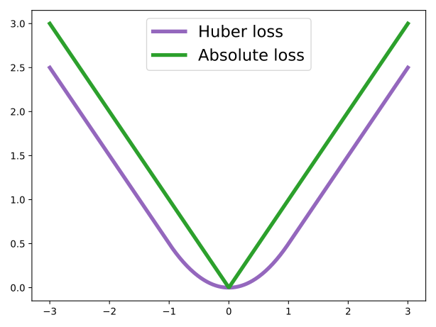
为从 Moreau 包络的视角说明平滑过程,我们展示如何对 -范数进行平滑。此时可得到 Moreau 包络的解析表达式。To illustrate smoothing from the Moreau envelope perspective, we show how to smooth the -norm. In this case, we obtain an analytical expression for the Moreau envelope.
例 13.1.5(通过下确卷积平滑 -范数)。Example 13.1.5 (Smoothing the -norm via infimal convolution).
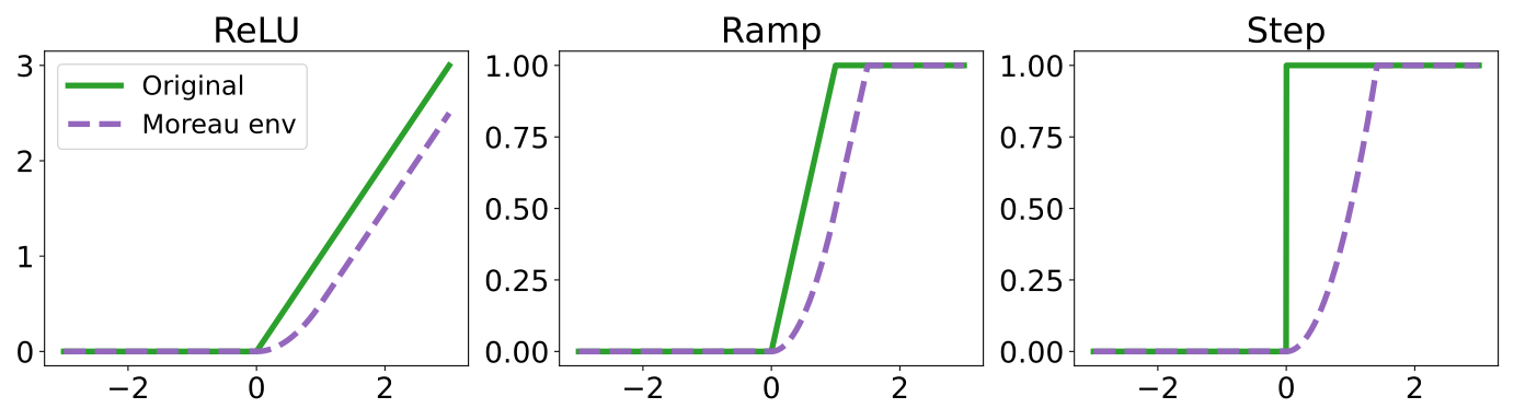
我们还在图 13.2 中表明,非凸函数的 Moreau 包络可以借助数值方法近似计算。We also illustrate in Fig. 13.2 that the Moreau envelope of nonconvex functions can be approximately computed numerically.
13.1.3 向量值函数Vector-valued functions
Moreau 包络由 定义,因此仅适用于标量值函数 。为把 Moreau 包络推广到向量值函数 ,其中 ,且对 有 ,我们可以选择对每个 分别进行平滑,从而定义The Moreau envelope is defined by . As such, it is limited to scalar-valued functions . To extend the Moreau envelope to vector-valued functions , where and for , we may choose to smooth each separately to define
其中where
这一做法需要求解 个各自独立的极小化问题,并对每个输出坐标 分别做平滑。由命题 2.3.16 可知, 沿任意方向 的 VJP 即为This approach requires to solve separate minimization problems and performs the smoothing of each output coordinate independently. From Proposition 2.3.16, we then have that the VJP of with any direction is
在 这一特殊情形下,可得In the particular case , we obtain
文献 [171] 提出了另一种方案。回顾一下,对可微函数 , 沿方向 的 VJP 为An alternative was proposed by [171]. For a differentiable function , we recall that the VJP of with a direction reads
其中我们定义了标量值函数 。于是,倘若 不可微,一个自然的思路便是:用 Moreau 包络的梯度 来近似其(假若存在的话)VJP :where we defined the scalar-valued function . As a result, if is non-differentiable, a natural idea is to approximate its VJP (had it existed) by the gradient of the Moreau envelope
| (13.2) |
这样只需解一个优化问题,与输出个数 无关;而且当 时,还能把 作为一种特殊情形包含进来。This requires solving a single optimization problem, independently of the number of outputs . Moreover, for , this recovers as a special case.
原则上,这一方案使我们能够对层中使用 Moreau 包络的神经网络执行反向模式自动微分(梯度反向传播)。事实上,由命题 13.1.3, 沿方向 的近似 VJP 由下式给出This approach allows in principle to perform reverse-mode autodiff (gradient backpropagation) on a neural network whose layers use the Moreau envelope. Indeed, following Proposition 13.1.3, the approximate VJP of with a direction is given by
其中 是式 13.2 中极小化问题的解。但需要强调,这一极小化问题在一般情况下可能难以求解:执行梯度反向传播时,方向 未必非负,因此即便每个 都是凸的,式 13.2 中所极小化的函数仍可能是非凸的。另一个隐患是:方向 会影响平滑强度,而按理说,无论是否计算函数的 VJP,我们都应能对该函数做平滑。举例来说,在 这一特殊情形下,容易验证:当 时,可得where is the solution of the minimization problem in Eq. 13.2. However, we emphasize that this minimization problem could be difficult to solve in general. Indeed, when performing gradient backpropagation, the direction is not necessarily non-negative, therefore the function being minimized in Eq. 13.2 could be nonconvex, even if each is convex. Another potential caveat is that the direction influences the smoothing strength, while in principle we should be able to smooth a function independently of whether we compute its VJP or not. To see that, for example in the particular case , one easily checks that for , we get
用 Moreau 包络(更一般地说,用下确卷积)平滑向量值函数,仍是尚待探索的研究方向。第 14 章将说明,用卷积做平滑能更自然地处理向量值函数。Smoothing vector-valued functions by Moreau envelope (or more generally, by infimal convolution) remains an open area of research. We will see in Chapter 14 that smoothing by convolution more naturally supports vector-valued functions.
13.2 Legendre–Fenchel 变换与凸共轭13.2 Legendre–Fenchel transforms, convex conjugates
Legendre-Fenchel 变换又称凸共轭,它把函数 变为一个新函数,记作 。由于它在对偶平滑方法中举足轻重,下面我们详细加以回顾。The Legendre-Fenchel transform, a.k.a. convex conjugate, is a way to turn a function into a new function, denoted . We now review it in detail, as it plays a major role for the dual approach to smoothing.
13.2.1 定义Definition
考虑如下形式的一类仿射函数Consider the class of affine functions of the form
这些函数由斜率 与截距 参数化。现设 固定。给定函数 , 的仿射下界即所有形如 的函数,其中 对所有 均满足These functions are parametrized by their slope and their intercept . Now, suppose we fix . Given a function , affine lower bounds of are all the functions of such that satisfies for all ,
最紧的下界由 定义,使得The tightest lower bound is then defined by such that
其中,我们记得 的定义域定义为where we recall that the domain of is defined by
由此引出 Legendre-Fenchel 变换的定义,又称凸共轭。This leads to the definition of Legendre-Fenchel transform, a.k.a. convex conjugate.
定义 13.2.1(Legendre-Fenchel 变换,凸共轭)。Definition 13.2.1 (Legendre-Fenchel transform, convex conjugate).
我们使用 而非 ,以表明 可能为 。依据前述讨论, 是 斜率为 的最紧仿射下界的截距。图 13.3 对此作了图示。We use a rather than a to indicate that is potentially . Following the previous discussion, is the intercept of the tightest affine lower bound with slope of . This is illustrated in Fig. 13.3.
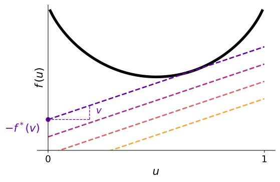
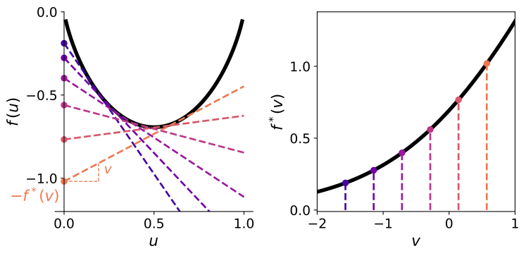
Legendre-Fenchel 变换是一种函数变换,因为它生成一个新的函数 。它可以视为函数的一种对偶表示:我们不必再用凸函数 在 上的图像 来表示它,而可以用一族切线来表示它:对 ,这些切线的斜率为 、截距为 ,如图 13.4 所示。正如“凸共轭”这一名称所示,即便原函数不是凸的,它也是凸的。The Legendre-Fenchel transform is a function transformation, as it produces a new function . It can be seen as a dual representation of a function: instead of representing a convex function by its graph for , we can represent it by the set of tangents with slope and intercept for , as illustrated in Fig. 13.4. As the name “convex conjugate” indicates, it is convex, even if the original function is not.
13.2.2 闭式示例Closed-form examples
计算 需要求解一个极大化问题;若对 不加任何假设,一般情形下这往往颇为棘手。不过,在某些情形下仍可求得解析表达式,下面举例说明。Computing involves the resolution of a maximization problem, which could be difficult in general without assumption on . In some cases, however, we can compute an analytical expression, as we now illustrate.
例 13.2.2(解析共轭示例)。Example 13.2.2 (Analytical conjugate examples).
约束定义域Constraining the domain
我们可以借助取值于扩展实数轴 的指示函数来施加约束,We can incorporate constraints using an indicator function with values in the extended real line ,
例 13.2.3(约束的引入)。Example 13.2.3 (Incorporating constraints).
13.2.3 性质Properties
凸共轭具有若干有用的性质,现总结如下。The conjugate enjoys several useful properties, that we now summarize.
命题 13.2.4(凸共轭的性质)。Proposition 13.2.4 (Convex conjugate properties).
证明 13.2.5。Proof 13.2.5.
- 1.
此结论源于如下事实:若 关于 为凸,则 为凸。注意,即便 关于 非凸,该结论依然成立。此处 关于 为仿射,因而关于 为凸。This follows from the fact that is convex if is convex in . Note that this is true even if is nonconvex in . Here, , which is affine in and therefore convex in .
- 2.
此结论由定义 13.2.1 直接得出。This follows immediately from Definition 13.2.1.
- 3.
此结论由 Danskin 定理得出,该定理已在 11.2 节中回顾。另一种理解方式,是注意到This follows from Danskin’s theorem, reviewed in Section 11.2. Another way to see this is by observing that
其中 。将两式相减,即得where . Subtracting the two, we obtain
现在,利用 的凸性以及定义 15.4.10,可得 。Now, using that is convex and Definition 15.4.10, we obtain that .
- 4.
例如参见 [15, 命题 16.10]。See, e.g., [15, Proposition 16.10].
- 5.
参见 [33, 3.3 节]。See [33, Section 3.3].
13.2.4 共轭运算法则Conjugate calculus
推导凸共轭的表达式一般可能相当困难,但在某些情形下,可以借助简单的法则,由其他共轭推导出所需的共轭。While deriving a convex conjugate expression can be difficult in general, in some cases, it is possible to use simple rules to derive conjugates in terms of other conjugates.
命题 13.2.6(共轭运算法则)。Proposition 13.2.6 (Conjugate calculus rules).
13.2.5 快速 Legendre 变换Fast Legendre transform
当解析表达式不可用时,可借助数值方案近似计算该变换/共轭。当 为凸时,由于 为凹,定义 13.2.1 中的极大化即为凹函数的极大化。因此,借助经典的约束优化迭代算法,如投影梯度下降(16.3 节)或条件梯度法(又称 Frank-Wolfe 算法 [100]),可在多项式时间内以任意精度算出该共轭。若不对 作凸性假设,则 可近似为When an analytical expression is not available, we can resort to numerical schemes to approximately compute the transform / conjugate. When is convex, because is concave, the maximization in Definition 13.2.1 is that of a concave function. Therefore, the conjugate can be computed to arbitrary precision in polynomial time using classical iterative algorithms for constrained optimization such as projected gradient descent (Section 16.3) or conditional gradient a.k.a. Frank-Wolfe [100]. Without convexity assumption on , can be approximated by
其中 是取值的离散网格。随后,我们可以利用线性时间 Legendre 变换算法 [123],针对若干个输入 计算对应的 ,其中 是另一个离散网格。其复杂度为 ,随网格规模线性增长。然而,网格规模通常为 ,即在 个维度上各取 个均匀分布的点。因此,该方法仅限于低维情形,例如 。where is a discrete grid of values. We can then compute for several inputs using the linear-time Legendre transform algorithm [123], where is another discrete grid. The complexity is , which is linear in the grid sizes. However, the grid sizes are typically , for equally-distributed points in each of the dimensions. Therefore, this approach is limited to small-dimensional settings, e.g., .
13.3 对偶方法13.3 Dual approach
前面我们介绍了如何通过与原始空间中的正则化项 做下确卷积来平滑一个函数。现在,我们介绍另一种做法:改为对函数的 Legendre-Fenchel 变换(凸共轭)进行正则化,从而平滑该函数。这种对偶的等价方法在数学上往往更为方便。Previously, we presented how to smooth a function by performing its infimal convolution with a primal-space regularization . We now present how to smooth a function by regularizing its Legendre-Fenchel transform (convex conjugate) instead. This dual, equivalent approach, is often mathematically more convenient.
13.3.1 强凸性与光滑性之间的对偶性Duality between strong convexity and smoothness
我们首先陈述一个众所周知的结果,本节的全部内容都建立在它之上:光滑性与强凸性彼此对偶 [96, 103, 18, 215]。We begin by stating a well-known result that will underpin this whole section: smoothness and strong convexity are dual to each other [96, 103, 18, 215].
命题 13.3.1(强凸性与光滑性之间的对偶性)。Proposition 13.3.1 (Duality between strong convexity and smoothness).
关于光滑性与强凸性这两个概念的回顾,见 15.4 节。表 13.2 给出了强凸与光滑共轭对的两个例子。For a review of the notions of smoothness and strong convexity, see Section 15.4. We give two examples of strongly-convex and smooth conjugate pairs in Table 13.2.
| 函数Function | 范数Norm | 定义域Domain | 共轭Conjugate | 对偶范数Dual norm | 对偶定义域Dual domain |
|---|---|---|---|---|---|
13.3.2 通过对偶正则化进行平滑Smoothing by dual regularization
光滑性与强凸性之间的对偶性提示了一种平滑函数 的通用方法,即经由对偶空间来完成。The duality between smoothness and strong convexity suggests a generic approach in order to smooth a function , by going through the dual space.
- 1.
计算共轭 :Compute the conjugate :
- 2.
为共轭加上强凸正则化项 :Add strongly-convex regularization to the conjugate:
(13.3) - 3.
再回到原始空间,即计算 的共轭:Go back to the primal space, by computing the conjugate of :
注意, 与 属于不同的空间,即 与 。根据命题 13.3.1,若 为 -强凸,则 为 -光滑。此外,根据命题 13.2.4,即便 非凸, 也是凸的。因此, 是 的一个光滑且凸的松弛。Note that and belong to different spaces, i.e., and . Following Proposition 13.3.1, if is -strongly convex, then is -smooth. Furthermore, following Proposition 13.2.4, is convex, even if is nonconvex. Therefore, is a smooth and convex relaxation of .
步骤 与 最具挑战性,因为二者都需要推导共轭。一般情况下解析解可能并不存在,但在某些简单情形下确实存在,下面我们对此加以说明。Steps and are the most challenging, as they both require the derivation of a conjugate. While an analytical solution may not exist in general, in some simple cases, there is, as we now illustrate.
例 13.3.2(通过对偶正则化平滑 -范数)。Example 13.3.2 (Smoothing the -norm via dual regularization).
ReLU 函数也可以用类似的方式平滑,我们将在 13.4 节中更详细地说明这一点。ReLU functions can be smoothed out in a similar way, as we see in more details in Section 13.4.
对偶方法使我们能够方便地借助原函数来界定平滑后的函数。The dual approach allows us to easily bound the smoothed function in terms of the original function.
命题 13.3.3(对平滑后的函数进行界定)。Proposition 13.3.3 (Bounding the smoothed function).
证明 13.3.4。Proof 13.3.4.
我们定义Let us define
其中我们回顾 。于是对任意 ,都有where we recall that . We then have for all
类似地,Similarly,
结合二者,并利用对任意 都有 这一事实,我们得到Combining the two with for all , we obtain
注 13.3.5(该梯度几乎处处可微)。Remark 13.3.5 (The gradient is differentiable almost everywhere).
13.3.3 原始正则化与对偶正则化的等价性Equivalence between primal and dual regularizations
至此,我们已经看到两种获得函数 的光滑近似的方法。第一种方法基于下确卷积 ,其中 表示原始正则化;第二种方法则基于用某个对偶正则化 对 的 Legendre-Fenchel 变换(凸共轭) 进行正则化,以定义 。结果表明,这两种方法是等价的。So far, we saw two approaches to obtain a smooth approximation of a function . The first approach is based on the infimal convolution , where denotes primal regularization. The second approach is based on regularizing the Legendre-Fenchel transform (convex conjugate) of with some dual regularization , to define . It turns out that both approaches are equivalent.
命题 13.3.6(原始正则化与对偶正则化的等价性)。Proposition 13.3.6 (Equivalence between primal and dual regularizations).
证明 13.3.7。Proof 13.3.7.
我们有We have
若 与 为凸,则 [18, 定理 4.17]。利用 与 ,并考虑到 与 (因为二者既凸又闭,见命题 13.2.4),即可得到所需结果。If and are convex, we have [18, Theorem 4.17]. Using and gives the desired result using that and since both are convex and closed (see Proposition 13.2.4).
特别地,取 ,这表明 Moreau 包络可以等价地写成In particular, with , this shows that the Moreau envelope can equivalently be written as
鉴于原始方法与对偶方法之间的等价性,采用哪一种方法主要取决于具体情形下数学上或算法上的便利性。Given the equivalence between the primal and dual approaches, using one approach or the other is mainly a matter of mathematical or algorithmic convenience, depending on the case.
13.3.4 正则化的缩放Regularization scaling
对偶方法Dual approach
若 是 -强凸的,则 构成原函数 的一个 -光滑近似。为控制该近似的光滑程度,我们用 作正则化,其中 ,并定义If is -strongly convex, then is a -smooth approximation of the original function . To control the smoothness of the approximation, we regularize with for , defining
据此,梯度可表示为Consequently, the gradient is given by
该表述对任意闭凸的 均成立。平滑所带来的近似误差可用命题 13.3.3 加以量化。只要对所有 都有 ,便有This formulation works for any closed convex . The approximation error induced by the smoothing can be quantified using Proposition 13.3.3. Provided that for all , we have
注 13.3.8(齐次情形)。Remark 13.3.8 (Homogeneous case).
原始方法Primal approach
根据定义 13.1.2,若采用对偶正则化 ,其中 控制正则化强度,并假设 为凸,则对应的原始正则化为 ,且有Following Definition 13.1.2, if we use dual regularization , where controls the regularization strength, assuming is convex, the corresponding primal regularization is and we have
在 这一特殊情形下,可得In the particular case , we have
由此得到We therefore get
13.3.5 广义熵Generalized entropies
当 为离散概率分布时,对偶正则化 的一个自然选择是负熵函数,亦称负熵。由于负熵在平滑的 max 算子中扮演重要角色,此处对其详加讨论。A natural choice of dual regularization , when is a discrete probability distribution, is a negative entropy function, also known as negentropy. Since negentropies play a major role in smoothed max operators, we discuss them in detail here.
信息量与熵Information content and entropy
熵函数衡量的是随机变量、亦或分布的“意外”程度。要定义熵,首先须定义事件 的信息量 。若事件的概率为 ,则该函数应返回 ,因为此时并无意外;反之,若事件的概率为 ,信息量应取到最大值,因为此时意外程度最大。此外,事件 越可能发生,其意外程度便越小。因此,当 增大时, 应当减小。此处略微滥用记号,我们也把随机变量 的取值 的信息量记作事件 的信息量,An entropy function measures the amount of “surprise” of a random variable or equivalently of a distribution. To define an entropy, we must first define the information content of an event . The value returned by such a function should be if the probability of the event is , as there is no surprise. Conversely, information content should attain its maximal value if the probability of the event is , as it is maximally surprising. Furthermore, the more probable an event is, the less surprising it is. Therefore, when increases, should decrease. Overloading the notation, we also write the information content of the outcome of a random variable as the information content of the event ,
有了信息量函数,便可把随机变量 的熵 定义为信息量的期望,Given an information content function, we can then define the entropy of a random variable as the expected information content,
信息量的定义不同,导出的熵的定义也便不同。Different definitions of information content lead to different definitions of entropy.
Shannon 熵Shannon’s entropy
满足上述各项标准的一种信息量定义是A definition of information content satisfying the criteria above is
事实上,、 与 在 上均为递减函数。采用这一信息量定义,便得到 Shannon 熵 [184]Indeed, , and is a decreasing function over . Using this information content definition leads to Shannon’s entropy [184]
据此,我们可以把离散概率分布 的 Shannon 熵定义为We can therefore define the Shannon entropy of a discrete probability distribution as
并将相应的负熵用作正则化and use the corresponding negentropy as regularization
该函数关于 在 上是强凸的;但它并非在 上强凸,因为后者不是有界集,例如参见 [26, 命题 2]。由于式 13.3 将 加到 上,因此只要 ,我们便能以这样选取的 来平滑函数 。The function is strongly convex w.r.t. over . However, it is not strongly convex over , since this is not a bounded set; see for instance [26, Proposition 2]. Since is added to in Eq. 13.3, we can therefore use this choice of to smooth out a function if .
Gini 熵Gini’s entropy
作为另一种选择,我们也可以把信息量定义为As an alternative, we can define information content as
其中 因子是为了后文在数学上处理方便。它同样满足信息量函数的各项要求。事实上:i)当 时,;ii)当 时, 取到最大值 ;iii)该函数关于 递减。采用这一信息量定义,便得到 Gini 熵,又称 Gini 指数 [78]The factor is for later mathematical convenience. This again satisfies the criteria of an information content function. Indeed, i) when , ii) when , attains its maximum of iii) the function is decreasing w.r.t. . Using this information content definition leads to Gini’s entropy a.k.a. Gini index [78]
我们可以借助 Gini 负熵,对所有 定义We can use Gini’s negative entropy to define for all
该函数关于 在 上是强凸的。因此只要 ,我们便能以这样选取的 来平滑函数 。这意味着,可用 Gini 熵平滑的函数集合,大于可用 Shannon 熵平滑的函数集合。The function is strongly convex w.r.t. over . We can therefore use this choice of to smooth out a function if . This means that the set of functions that we can smooth out with Gini entropy is larger than the set of functions we can smooth out with Shannon entropy.
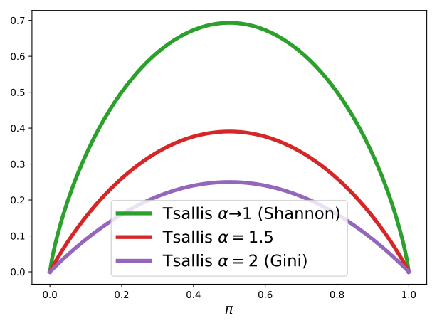
Tsallis 熵Tsallis entropies
给定 ,一种更一般的信息量定义为Given , a more general information content definition is
采用这一信息量定义,便得到 Tsallis 熵 [197]Using this definition leads to the Tsallis entropy [197]
Tsallis 熵在 的极限下退化为 Shannon 熵,而当 时则退化为 Gini 熵。借助 Tsallis 负熵,我们可以对任意 定义The Tsallis entropy recovers the Shannon entropy in the limit and the Gini entropy when . We can use the Tsallis negative entropy to define for all
其中 为 -范数()where is the -norm for ()
于是so that
(Shannon 熵)、 与 (Gini 熵)对应的 Tsallis 熵如图 13.5 和图 13.6 所示。Tsallis entropies for (Shannon entropy), and (Gini entropy) are illustrated in Fig. 13.5 and Fig. 13.6.
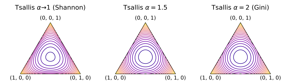
广义熵的定义与性质Definition and properties of generalized entropies
至此,我们已看到如何将熵定义为期望信息量。然而,广义熵 [53, 89] 未必需要采取这种形式。我们沿用 [28] 的定义。So far, we saw how to define an entropy as the expected information content. However, generalized entropies [53, 89] do not necessarily need to take this form. We follow the definition of [28].
定义 13.3.9(熵函数)。Definition 13.3.9 (Entropy function).
由该定义可知, 非负,且均匀分布是其唯一的极大值点 [28, 命题 4]。这正是人们对熵函数的预期。平方 -范数熵便是一例 [28]This definition implies that is non-negative and is uniquely maximized by the uniform distribution [28, Proposition 4]. This is indeed what we expect from an entropy function. An example is the squared -norm entropy [28]
由于平方 -范数在 时强凸 [8],该熵在 时强凹,因而可用于平滑函数。Since the squared -norm is strongly convex for [8], this entropy is strongly concave for and can therefore be used to smooth out functions.
下面我们说明如何应用这些技术,计算平滑的 ReLU 与平滑的 max 算子,以及阶跃函数与 argmax 算子的连续松弛。We now illustrate how to apply these techniques to compute smoothed ReLUs and smoothed max operators, as well as continuous relaxations of step functions and argmax operators.
13.4 平滑的 ReLU 函数13.4 Smoothed ReLU functions
为演示本章所讨论的平滑技术如何应用,我们先说明如何平滑 ReLU 函数。ReLU 函数定义为To demonstrate the application of the smoothing techniques discussed in this chapter, we begin by explaining how to smooth the ReLU function. The ReLU function is defined by
我们记得,要用对偶方法平滑函数 ,需先求其共轭 ,对其施加正则化项 得到 ,再通过计算 得到 。We recall that in order to smooth a function by the dual approach, we calculate its conjugate , add regularization to it to obtain and then obtain by computing .
这里我们希望平滑 。它的凸共轭为Here, we wish to smooth out . Its convex conjugate is
要弄清其中缘由,我们观察到To notice why, we observe that
| (13.4) |
确实,目标函数关于 是线性的,故最大值必在 的某个极点处取得,于是可将约束 换成 。这说明 ReLU 恰是 的支撑函数。而支撑函数的共轭为指示函数,故确实得到 。于是有Indeed, since the objective is linear in , the maximum is attained at one of the extreme points of , so that we can replace the constraint with . This shows that the ReLU is exactly the support function of . Since the conjugate of the support function is the indicator function, we indeed obtain . We therefore have
并且,对 的某种选取,我们需要能够计算and for some choice of , we need to be able to compute
softplusThe softplus
若采用正则化项 ,它源于使用 Shannon 负熵 并取 ,则得到If we use the regularizer , which comes from using Shannon’s negentropy with , we obtain
这一结果是命题 13.5.4 的一个特例。This result is a special case of Proposition 13.5.4.
稀疏 plus(sparseplus)The sparseplus
若采用正则化项 ,它源于使用 Gini 负熵并取 与 ,则得到If we use the regularizer , which comes from using Gini’s negentropy with with , we obtain
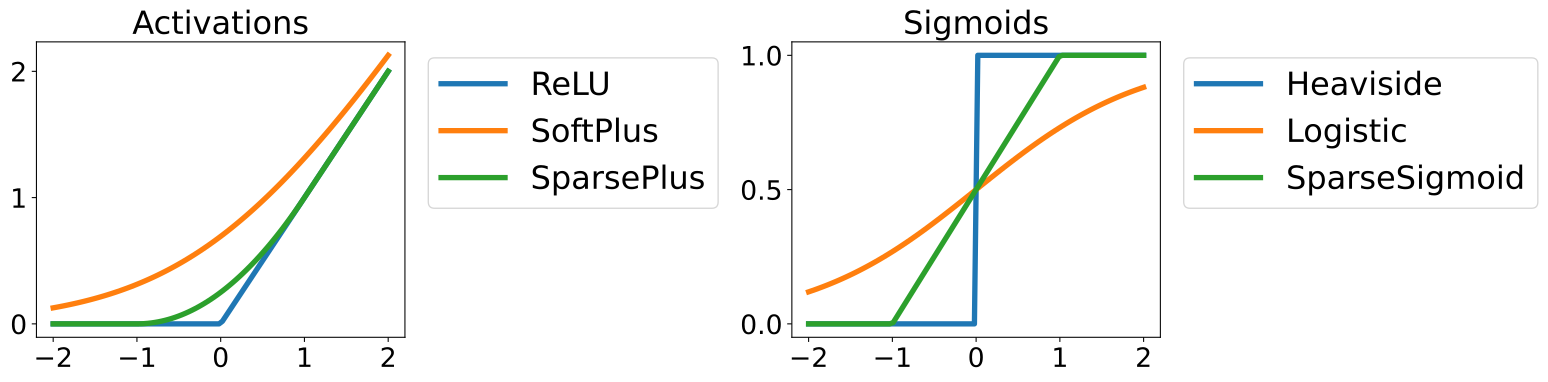
softplus 与 sparseplus 的对比见图 13.8(左图)。See Fig. 13.8 (left figure) for a comparison of softplus and sparseplus.
13.5 平滑的 max 算子13.5 Smoothed max operators
作为本章所讨论的平滑技巧的一个更精细的应用,我们说明如何平滑 max 算子。平滑的 max 算子将平滑的 ReLU 函数作为特例包含在内。As a more elaborate application of the smoothing techniques discussed in this chapter, we explain how to smooth max operators. Smoothed max operators include smoothed ReLU functions as a special case.
13.5.1 定义与性质Definition and properties
略微重载记号,给定向量 ,我们将其最大值定义为With a slight notation overloading, given a vector , we define its maximum as
为得到 的光滑近似 ,我们再次采用对偶方法。 的共轭为To obtain a smooth approximation of , we again apply the dual approach. The conjugate of is
要理解其中缘由,我们观察到概率单纯形 的极点是标准基向量 。由于目标函数是线性的,于是有To notice why, we observe that the vertices of the probability simplex are the standard basis vectors . Since the objective is linear, we then have
换言之,max 算子恰是 的支撑函数。由于支撑函数的共轭为指示函数,我们确实得到 。因此可以将其写成In other words, the maximum operator is exactly the support function of . Since the conjugate of the support function is the indicator function, we indeed obtain . We can therefore write
以及and
平滑的 max 算子 在神经网络中可能很有用,例如可用作平滑的最大池化层。其性质已在 [132, 引理 1] 中研究,为方便起见我们在此回顾。The smoothed max operator can be useful in a neural network, for example as a smoothed max pooling layer. Its properties have been studied in [132, Lemma 1], as we recall here for convenience.
命题 13.5.1( 的性质)。Proposition 13.5.1 (Properties of ).
这些性质在 [132] 中被用于构造可微的动态规划。下面我们考虑 的两种可能选择,它们分别引出图 13.7 所示的 softmax 与 sparsemax 算子。These properties are leveraged in [132] to create differentiable dynamic programs. We consider in the following two possible choices of leading to the softmax and sparsemax operators illustrated in Fig. 13.7.
平滑的 min 算子Smoothed min operators
min 算子可以用 max 算子表示,因为对所有 ,The minimum operator can be expressed in terms of the maximum operator, since for all ,
因此,给定平滑的 max 算子 ,我们可以很容易地将平滑的 min 算子定义为Given a smoothed max operator , we can therefore easily define a smoothed min operator as
13.5.2 化归为求根Reduction to root finding
对一般的强凸正则化项 计算 ,涉及在概率单纯形约束下求解一个极大化问题。为方便起见,我们定义记号Computing for a general strongly-convex regularization involves the resolution of a maximum over probability simplex constraints. For convenience, let us define the notation
下面的命题表明,我们可以把 的计算化归为求解一个涉及 的根方程。The following proposition shows that we can reduce computing to solving a root equation involving .
命题 13.5.2(将 的计算化归为求根)。Proposition 13.5.2 (Computing as root finding).
证明 13.5.3。Proof 13.5.3.
思路是保留非负约束为显式约束,而对概率单纯形的等式约束使用拉格朗日乘子。于是有The idea is to keep the non-negativity constraint explicit, but to use a Lagrange multiplier for the equality constraint of the probability simplex. We then have
这里我们利用了可以交换 与 的次序,因为 是凸—凹的,且 为仿射约束。梯度 由 Danskin 定理给出。根方程则来自对 求导并令其等于零。where we used that we can swap the and the , since is convex-concave and is an affine constraint. The gradient follows from Danskin’s theorem. The root equation follows from computing the derivative of and setting it to zero.
13.5.3 softmaxThe softmax
当 取 Shannon 负熵时,可得 就是 softmax,这一点已在 4.4.2 节中简要讨论过。When is Shannon’s negentropy, we obtain that is the softmax, already briefly discussed in Section 4.4.2.
命题 13.5.4(softmax 的解析表达式)。Proposition 13.5.4 (Analytical expression of the softmax).
证明 13.5.5。Proof 13.5.5.
由于 ,故有 (即非负约束是多余的)。于是由例 13.2.2 得 。根据命题 13.5.2,,其中 满足 。由于 ,我们需解 。由此得到 ,从而有 。Since , we have (i.e., the non-negativity constraint is redundant). From Example 13.2.2, we therefore have . From Proposition 13.5.2, where satisfies Since , we need to solve . We therefore get and therefore .
由于对所有 都有 ,依命题 13.5.1 可得,对所有 均有Since for all , following Proposition 13.5.1, we get for all
softmax 有一项独特之处:它支持结合律,而这一点并非所有 算子都具备。A unique property of the softmax, which is not the case of all operators, is that it supports associativity.
命题 13.5.6(softmax 的结合律)。Proposition 13.5.6 (Associativity of the softmax).
13.5.4 sparsemaxThe sparsemax
另一种选择是将 取为 Gini 负熵,由此便得到 sparsemax [129, 132]。Alternatively, choosing to be Gini’s negentropy leads to the sparsemax [129, 132].
命题 13.5.7(sparsemax 的变分表述)。Proposition 13.5.7 (Variational formulation of sparsemax).
证明 13.5.8。Proof 13.5.8.
这源于这样一个事实: 与 至多相差一个常数,再配方即可得证。This follows from the fact that is up to a constant equal to and completing the square.
因此,计算 sparsemax 时可以把 sparseargmax(即向概率单纯形上的欧几里得投影)当作一个基本构件。其具体计算方法将在 13.7 节中更详细地讨论。应用命题 13.5.2 则可得到另一种表述。Therefore, computing the sparsemax can use the sparseargmax (the Euclidean projection onto the probability simplex) as a building block. We discuss how to compute it in more detail in Section 13.7. Applying Proposition 13.5.2 gives an alternative formulation.
命题 13.5.9(以求根形式表示的 sparsemax)。Proposition 13.5.9 (Sparsemax as root finding).
证明 13.5.10。Proof 13.5.10.
首先计算 的表达式。令 的梯度为零并作截断,得到 。将 代回,得到 。第一部分由命题 13.5.2 得证。令关于 的导数为零,即得第二部分。First, we compute the expression of . Setting the gradient of to zero and clipping, we obtain . Plugging back, we obtain . Using Proposition 13.5.2 proves the proposition’s first part. Setting the derivative w.r.t. to zero gives the second part.
可以证明 [59, 48],精确解 由下式给出It can be shown [59, 48] that the exact solution is obtained by
| (13.5) |
其中 是使下式成立的最大 where is the largest such that
这里我们采用了记号 。作为另一种选择,也可以用二分法或关于 的梯度下降来近似计算 。and where we used the notation . As an alternative, we can also compute approximately using a bisection or by gradient descent w.r.t. .
对于 ,由于 ,我们有 。因此,根据命题 13.5.1,对所有的 ,可得For , since , we have Following Proposition 13.5.1, we therefore get for all
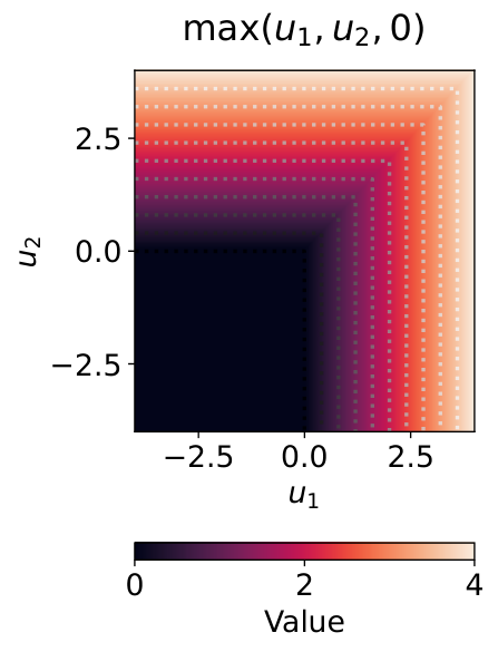
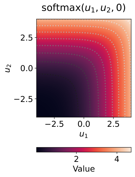
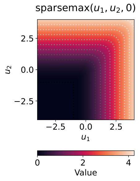
13.5.5 恢复平滑的 ReLU 函数Recovering smoothed ReLU functions
以向量 为输入,平滑的 max 算子便可恢复出平滑的 ReLU:Using the vector as input, the smoothed max operator recovers the smoothed ReLU:
其中我们定义了 。当 为 Shannon 负熵时,便恢复出 ;当 为 Gini 负熵时,则恢复出 ,我们正是用它来平滑 ReLU 的。where we defined . With being Shannon’s negentropy, we recover ; with being Gini’s negentropy, we recover , that we used to smooth the ReLU.
13.6 松弛的阶跃函数(S 形函数)13.6 Relaxed step functions (sigmoids)
下面转向构造阶跃函数的连续松弛。二值阶跃函数又称 Heaviside 阶跃函数,定义为We now turn to creating continuous relaxations of step functions. The binary step function, a.k.a. Heaviside step function, is defined by
由式 13.4,其变分形式为From Eq. 13.4, its variational form is
因此,我们可以定义该松弛We can therefore define the relaxation
注意,与平滑 ReLU 的情形不同,这里得到的是正则化的 argmax,而非正则化的 max。根据注 13.3.5,强凸正则化项 保证了 是 的 Lipschitz 连续函数,因而至少几乎处处可微,这一点与 不同。Notice that, unlike the case of the smoothed ReLU, it is a regularized argmax, not a regularized max. Following Remark 13.3.5, strongly convex regularization ensures that is a Lipschitz continuous function of and is therefore, at least, differentiable almost everywhere, unlike .
logistic 函数The logistic function
若采用正则化项 ,则得到如下闭式形式If we use the regularizer , we obtain the closed form
该函数处处可微。This function is differentiable everywhere.
稀疏 S 形函数The sparse sigmoid
作为另一种选择,若采用 ,则得到一个分段线性的 S 形函数,As an alternative, if we use , we obtain a piecewise linear sigmoid,
与 logistic 函数不同,它可以取到精确值 或 。然而,该函数有两个折角,在这些位置上函数不可微。Unlike the logistic function, it can reach the exact values or . However, the function has two kinks, where the function is non-differentiable.
平滑 ReLU 函数与 S 形函数之间的联系Link between smoothed ReLU functions and sigmoids
事实证明,上面介绍的三种 S 形函数(阶跃函数、logistic 函数、稀疏 S 形函数)都等于其对应平滑 ReLU 函数的导数:It turns out that the three sigmoids we presented above (step, logistic, sparsesigmoid) are all equal to the derivative of their corresponding smoothed ReLU function:
更一般地,and more generally
这是 Danskin 定理的一个推论;见例 11.2.5。图 13.8 展示了平滑 ReLU 函数与松弛阶跃函数(S 形函数)。This is a consequence of Danskin’s theorem; see Example 11.2.5. We illustrate the smoothed ReLU functions and relaxed step functions (sigmoids) in Fig. 13.8.
13.7 松弛的 argmax 算子13.7 Relaxed argmax operators
现在我们转向 argmax 算子,它是阶跃函数的推广。略微滥用记号,我们定义We now turn to argmax operators, which are a generalization of step functions. With a slight notation overloading, let us now define
其中 用于将任意整数 嵌入到 中。按照前面的讨论,可得变分形式where is used to embed any integer into . Following the previous discussion, we have the variational form
其中第二个等式利用了线性函数在单纯形的某个顶点处取得最大值这一事实。该变分形式提示我们定义如下松弛:where the second equality uses that a linear function is maximized at one of the vertices of the simplex. This variational form suggests to define the relaxation
同样,根据注 13.3.5,若 是强凸的,则 至少是 的一个几乎处处可微的函数。Again, following Remark 13.3.5, is guaranteed to be, at least, a differentiable almost everywhere function of if is strongly convex.
与 S 形函数类似,事实证明这些映射等于其对应平滑 max 算子的梯度:Similarly to sigmoids, it turns out that these mappings are equal to the gradient of their corresponding smoothed max operator:
这同样是 Danskin 定理的一个推论。This is again a consequence of Danskin’s theorem.
softargmaxThe softargmax
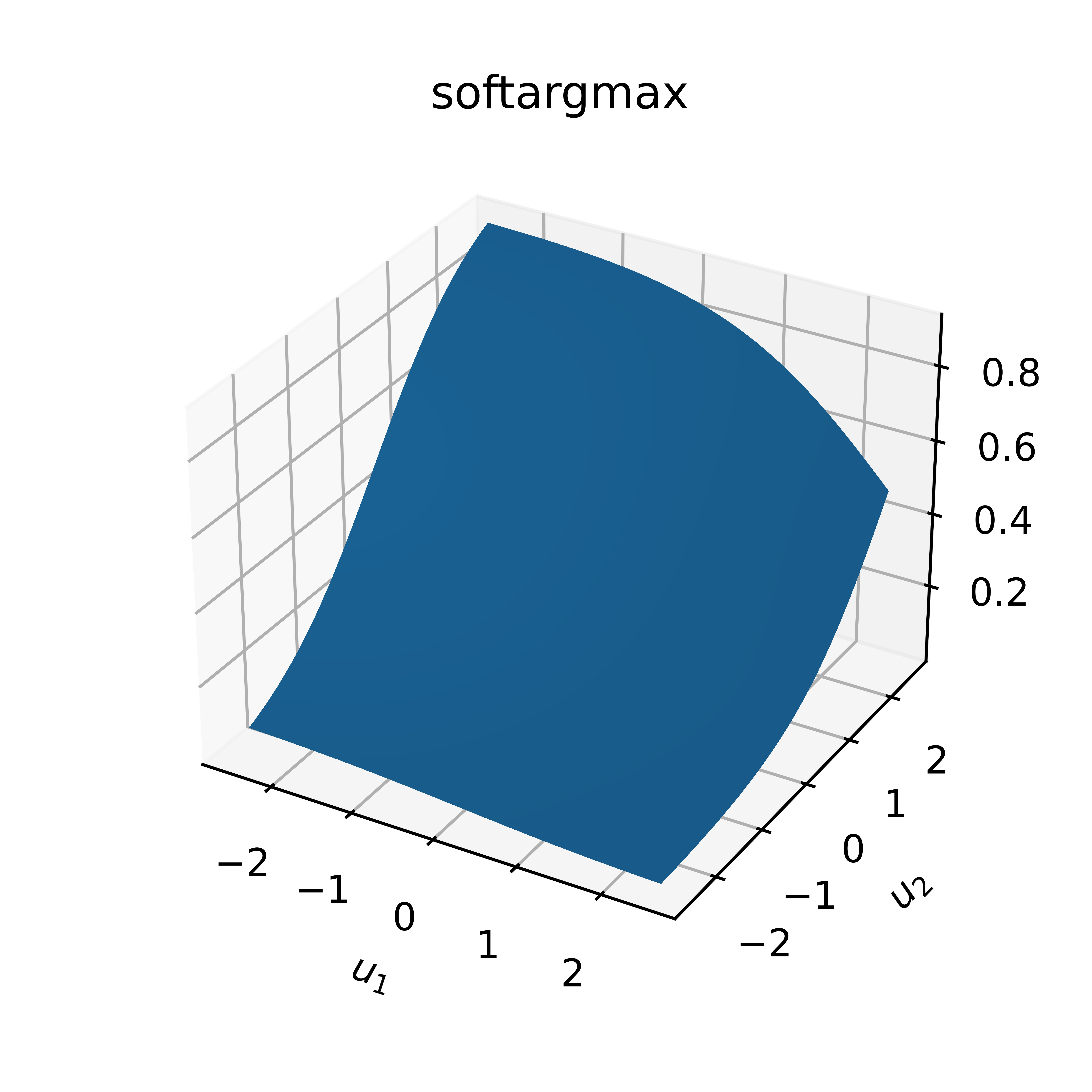
当采用 Shannon 负熵 时,我们得到When using Shannon’s negative entropy , we obtain
该函数处处可微。which is differentiable everywhere.
证明 13.7.1。Proof 13.7.1.
我们知道 以及 。对 求导得到 。We know that and that . Differentiating gives .
sparseargmaxThe sparseargmax
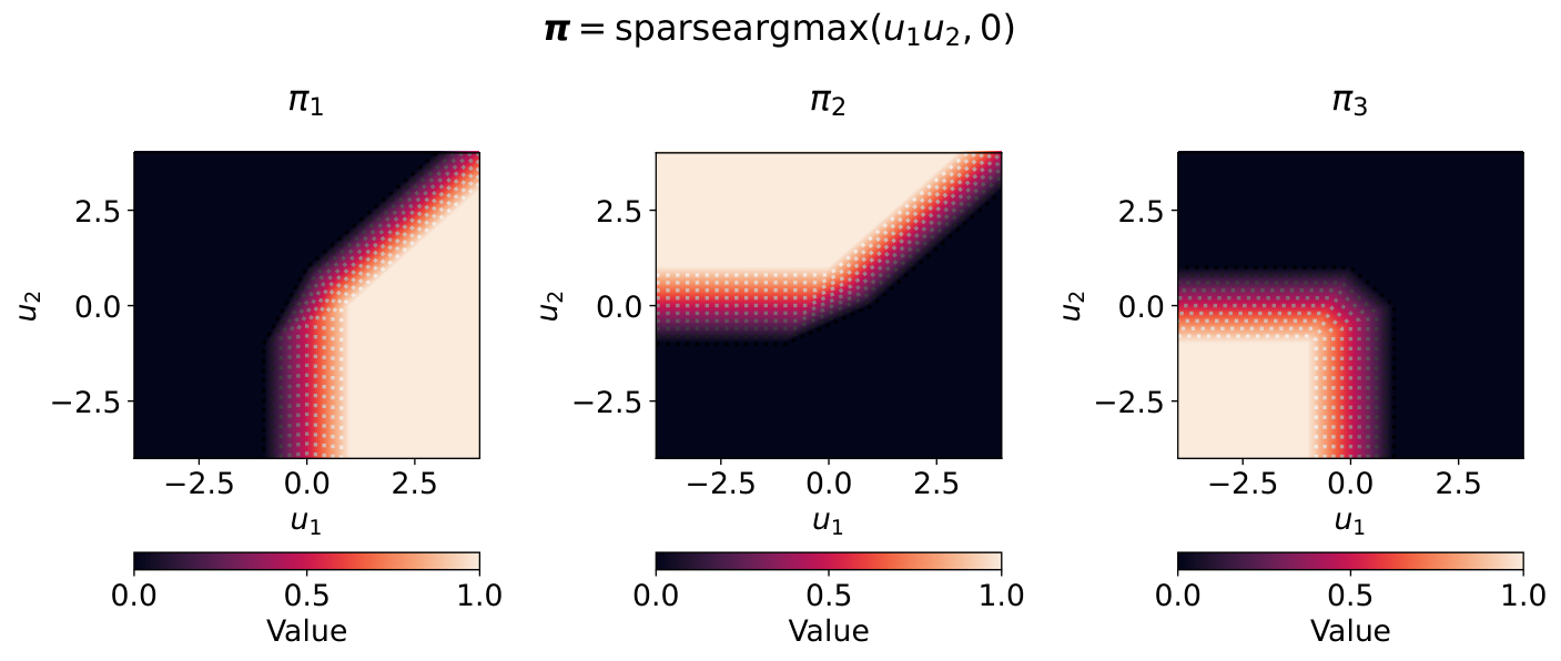
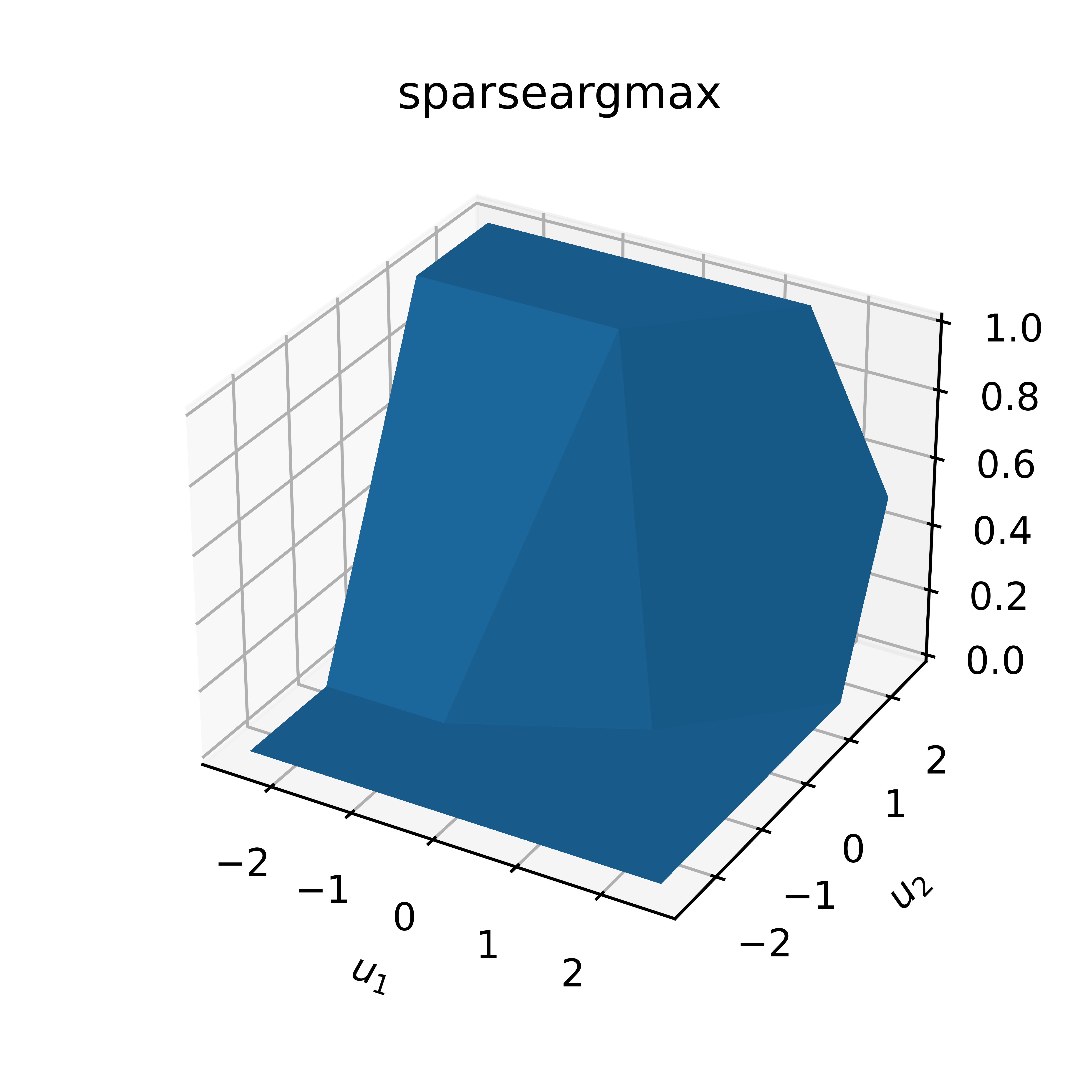
当采用 Gini 熵 (它与 相差一个常数)时,我们得到 sparseargmax [129]When using Gini’s entropy , which is up to a constant equal to , we obtain the sparseargmax [129]
它正是向概率单纯形上的欧几里得投影(另见 16.3 节)。向概率单纯形 上的欧几里得投影可以用类似寻找中位数的算法精确计算,其期望时间复杂度为 ,最坏情况时间复杂度为 [38, 135, 59, 48]。计算向概率单纯形上的欧几里得投影归结为计算式 13.5 中给出的 。一旦算出该值,便有which is nothing but the Euclidean projection onto the probability simplex (see also Section 16.3). The Euclidean projection onto the probability simplex can be computed exactly using a median-finding-like algorithm. The complexity is expected time and worst-case time [38, 135, 59, 48]. Computing the Euclidean projection onto the probability simplex boils down to computing given in Eq. 13.5. Once we computed it, we have
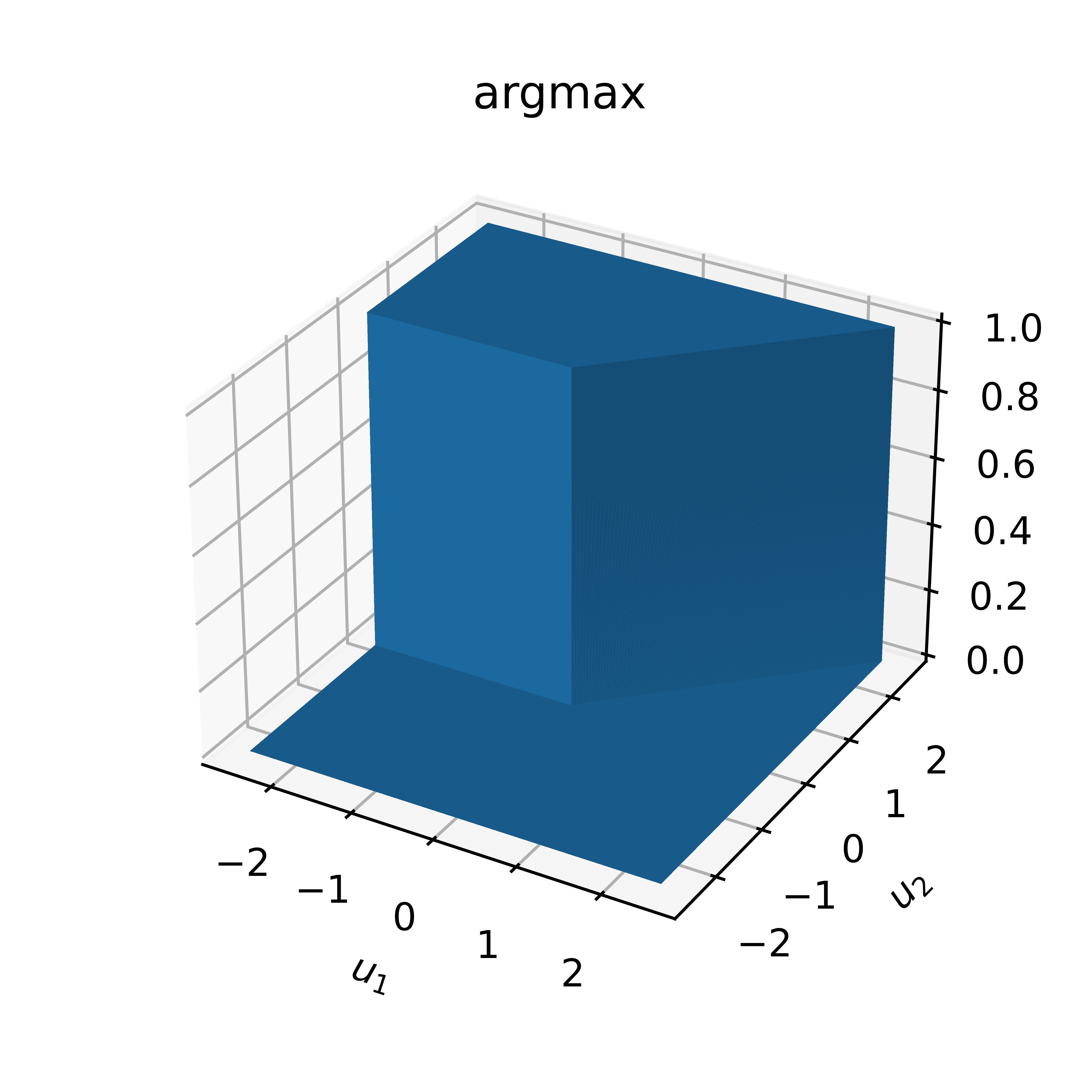
正如其名称所示,也如上式所示,sparseargmax 是稀疏的,但它只是几乎处处可微。注意,该算子最初被称为 sparsemax [129],但这是一个误称,因为它实际上是 argmax 的一种近似。因此,类比 softargmax,我们使用 sparseargmax 这一名称。图 13.9 与图 13.10 比较了 argmax、softmax 与 sparseargmax。As its name indicates, and as the above equation shows, sparseargmax is sparse, but it is only differentiable almost everywhere. Note that the operator is originally known as sparsemax [129], but this is a misnomer, as it is really an approximation of the argmax. Therefore, in analogy with the softargmax, we use the name sparseargmax. We compare the argmax, softmax and sparseargmax in Fig. 13.9 and Fig. 13.10.
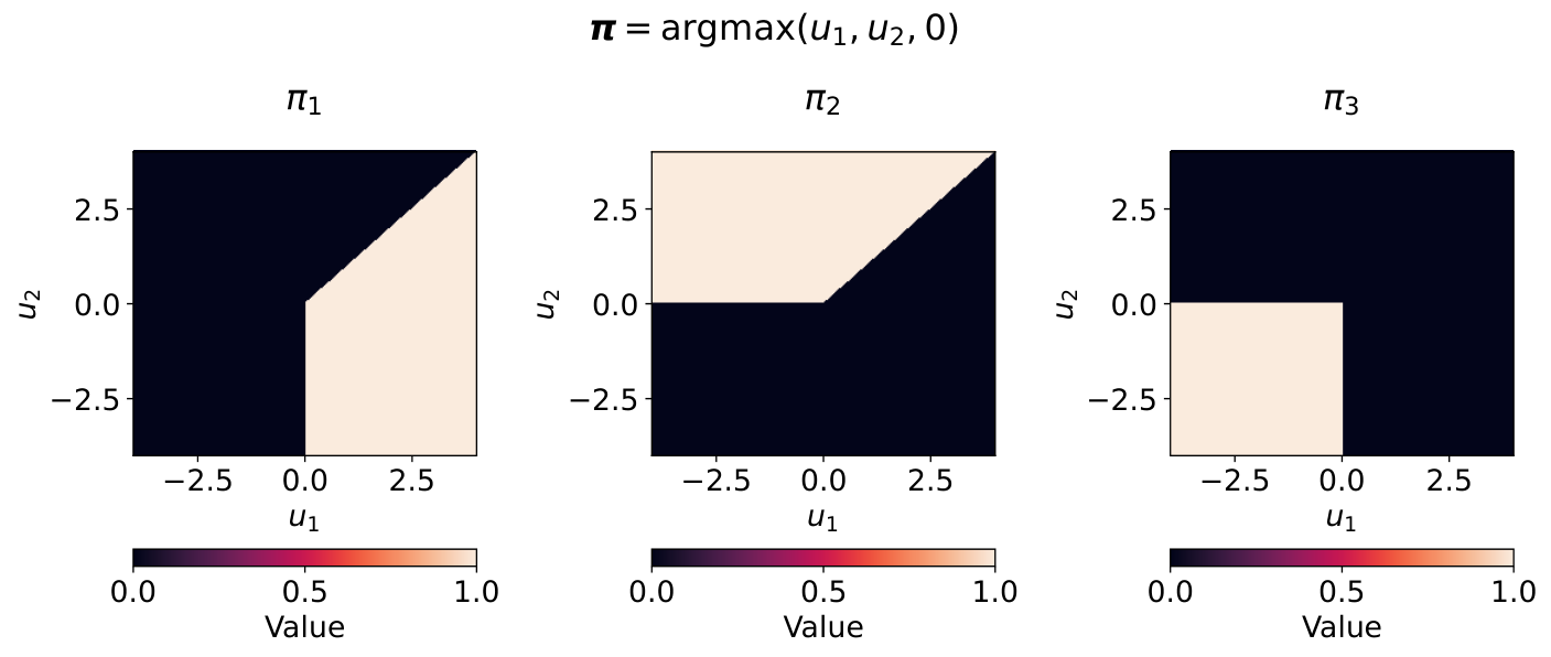
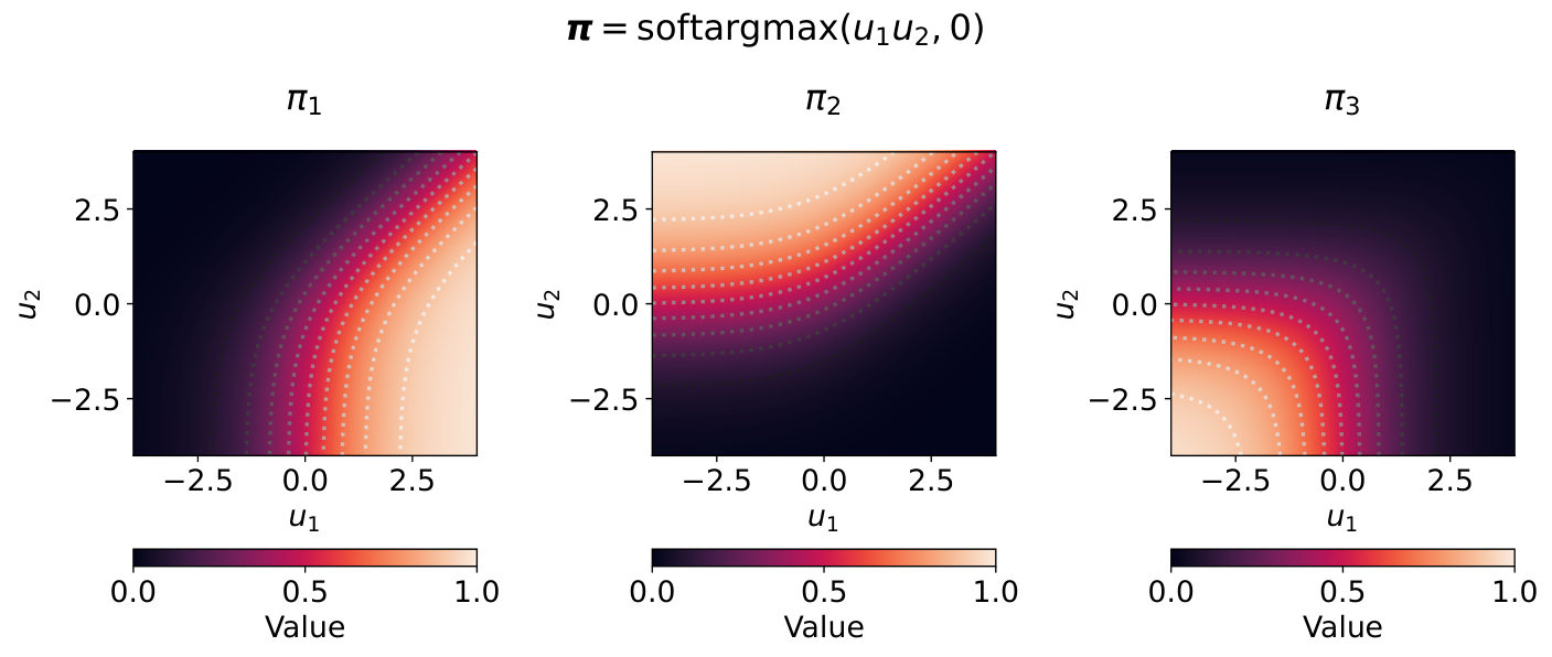
松弛的 argmin 算子Relaxed argmin operators
argmin 算子可以用 argmax 算子来表示,The argmin operator can be expressed in terms of the argmax operator,
因此,给定一个松弛的 argmax 算子 ,我们便可通过下式定义松弛的 argmin,Given a relaxed argmax operator , we can therefore define a relaxed argmin by
于是,对任意 ,都有We then have for all
13.8 小结13.8 Summary
- •
当函数 不可微(甚至不连续)时,一种合理的做法是用它的光滑近似(或连续松弛)来代替它。When a function is non-differentiable (or worse, discontinuous), a reasonable approach is to replace it by its smooth approximation (or continuous relaxation).
- •
我们回顾的第一种方法,是在 与原始正则化项 之间做下确卷积。Moreau 包络是其中的一个特例,只需取 即可得到。The first approach we reviewed is infimal convolution between and primal regularization . The Moreau envelope is a special case, obtained by using .
- •
我们回顾的第二种方法,是用某个对偶正则化项 对 的凸共轭 进行正则化。我们看到,当 时,原始方法与对偶方法彼此等价。The second approach we reviewed is regularizing the convex conjugate of with some dual regularization . We saw that the primal and dual approaches are equivalent when .
- •
Legendre-Fenchel 变换(又称凸共轭)可以视为函数的一种对偶表示:与其用 上的图像 来表示 ,不如用 上斜率为 、截距为 的一族切线来表示它。正如其名称所示,即便原函数并非凸函数,它也是凸的。The Legendre-Fenchel transformation, a.k.a. convex conjugate, can be seen as a dual representation of a function: instead of representing by its graph for , we can represent it by the set of tangents with slope and intercept for . As its name indicates, it is convex, even if the original function is not.
- •
我们展示了如何运用平滑技术来构造平滑的 ReLU 函数与平滑的 max 算子。我们还展示了,对它们求梯度便可得到广义的 S 形函数与 argmax 算子。We showed how to apply smoothing techniques to create smoothed ReLU functions and smoothed max operators. We also showed that taking their gradients allowed us to obtain generalized sigmoid functions and argmax operators.