第 8 章自动微分 · Automatic differentiation

8.1 计算链8.1 Computation chains

首先，考虑一条计算链（4.1.1 节），它表示一个函数 $f\colon\mathcal{S}_{0}\to\mathcal{S}_{K}$ ，该函数被表达为一串复合 $f\coloneqq f_{K}\circ\dots\circ f_{1}$ ，其中 $f_{k}\colon\mathcal{S}_{k-1}\to\mathcal{S}_{k}$ 。对 $f$ 的计算可以展开为一串操作To begin with, consider a computation chain (Section 4.1.1) representing a function $f\colon\mathcal{S}_{0}\to\mathcal{S}_{K}$ expressed as a sequence of compositions $f\coloneqq f_{K}\circ\dots\circ f_{1}$ , where $f_{k}\colon\mathcal{S}_{k-1}\to\mathcal{S}_{k}$ . The computation of $f$ can be unrolled into a sequence of operations

$\displaystyle{\bm{s}}_{0}$	$\displaystyle\in\mathcal{S}_{0}$
$\displaystyle{\bm{s}}_{1}$	$\displaystyle\coloneqq f_{1}({\bm{s}}_{0})\in\mathcal{S}_{1}$
	$\displaystyle\hskip 6.0pt\vdots$
$\displaystyle{\bm{s}}_{K}$	$\displaystyle\coloneqq f_{K}({\bm{s}}_{K-1})\in\mathcal{S}_{K}$
$\displaystyle f({\bm{s}}_{0})$	$\displaystyle\coloneqq{\bm{s}}_{K}.$	(8.1)

我们的目标是计算 $f$ 在给定输入 ${\bm{s}}_{0}$ 附近的变化。在前馈网络中，这相当于在参数固定时估计给定输入 ${\bm{s}}_{0}$ 的影响（我们将在后文看到如何估计关于参数 ${\bm{w}}$ 的变化）。Our goal is to compute the variations of $f$ around a given input ${\bm{s}}_{0}$ . In a feedforward network, this amounts to estimating the influence of a given input ${\bm{s}}_{0}$ for fixed parameters (we will see how to estimate the variations w.r.t. parameters ${\bm{w}}$ in the sequel).

雅可比矩阵Jacobian matrix

我们首先考虑完整雅可比 $\bm{\partial}f({\bm{s}}_{0})$ 的计算，如记号 $\bm{\partial}$ 所示，它被视为一个矩阵。根据命题 2.2.11，我们有We first consider the computation of the full Jacobian $\bm{\partial}f({\bm{s}}_{0})$ , seen as a matrix, as the notation $\bm{\partial}$ indicates. Following Proposition 2.2.11, we have

\bm{\partial}f({\bm{s}}_{0})=\bm{\partial}f_{K}({\bm{s}}_{K-1})\ldots\bm{\partial}f_{1}({\bm{s}}_{0}),

(8.2)

其中 $\bm{\partial}f_{k}({\bm{s}}_{k-1})$ 是在 ${\bm{s}}_{0},\ldots,{\bm{s}}_{K}$ 处计算得到的各中间函数的雅可比矩阵，如式 8.1 所定义。我们可能还想计算雅可比矩阵的转置where $\bm{\partial}f_{k}({\bm{s}}_{k-1})$ are the Jacobians of the intermediate functions computed at ${\bm{s}}_{0},\ldots,{\bm{s}}_{K}$ , as defined in Eq. 8.1. We may also want to compute the transpose of the Jacobian

\bm{\partial}f({\bm{s}}_{0})^{\top}=\bm{\partial}f_{1}({\bm{s}}_{0})^{\top}\ldots\bm{\partial}f_{K}({\bm{s}}_{K-1})^{\top}.

在这两种情形中，该方法的主要缺点都在于计算方面：计算完整的 $\bm{\partial}f({\bm{s}}_{0})$ 需要在内存中具体化各中间雅可比矩阵，并执行矩阵—矩阵乘积。然而在实践中，很少需要计算完整的雅可比矩阵。事实上，我们往往只需要右乘或左乘 $\bm{\partial}f({\bm{s}}_{0})$ 。这分别引出了前向模式自动微分与反向模式自动微分。In both cases, the main drawback of this approach is computational: computing the full $\bm{\partial}f({\bm{s}}_{0})$ requires materializing the intermediate Jacobians in memory and performing matrix-matrix multiplications. However, in practice, computing the full Jacobian is rarely needed. Indeed, oftentimes, we only need to right-multiply or left-multiply with $\bm{\partial}f({\bm{s}}_{0})$ . This gives rise to forward-mode and reverse-mode autodiff, respectively.

8.1.1 前向模式Forward-mode

现在我们把雅可比 $\partial f({\bm{s}}_{0})$ 解释为一个线性映射，正如非粗体的 $\partial$ 所示。根据命题 2.3.10， $\partial f({\bm{s}}_{0})$ 是各中间线性映射的组合，We now interpret the Jacobian $\partial f({\bm{s}}_{0})$ as a linear map, as the non-bold $\partial$ indicates. Following Proposition 2.3.10, $\partial f({\bm{s}}_{0})$ is the composition of the intermediate linear maps,

\partial f({\bm{s}}_{0})=\partial f_{K}({\bm{s}}_{K-1})\circ\ldots\circ\partial f_{1}({\bm{s}}_{0}).

在输入方向 ${\bm{v}}\in\mathcal{S}_{0}$ 上求值 $\partial f({\bm{s}}_{0})$ 时，可以像式 8.1 中的函数本身那样分解为若干中间计算Evaluating $\partial f({\bm{s}}_{0})$ on an input direction ${\bm{v}}\in\mathcal{S}_{0}$ can be decomposed, like the function Eq. 8.1 itself, into intermediate computations

$\displaystyle{\bm{t}}_{0}$	$\displaystyle\coloneqq{\bm{v}}$
$\displaystyle{\bm{t}}_{1}$	$\displaystyle\coloneqq\partial f_{1}({\bm{s}}_{0})[{\bm{t}}_{0}]$
	$\displaystyle\hskip 6.0pt\vdots$
$\displaystyle{\bm{t}}_{K}$	$\displaystyle\coloneqq\partial f_{K}({\bm{s}}_{K-1})[{\bm{t}}_{K-1}]$
$\displaystyle\partial f({\bm{s}}_{0})[{\bm{v}}]$	$\displaystyle\coloneqq{\bm{t}}_{K}.$

每个中间量 $\partial f_{k}({\bm{s}}_{k-1})[{\bm{t}}_{k-1}]$ 都相当于一个雅可比矩阵—向量乘积（JVP），并且可以与中间状态 ${\bm{s}}_{k}$ 的计算一同以前向方式执行。这也可以看作是用一个向量从右向左乘以式 8.2 所定义的矩阵。图 8.1 对此作了图示，算法 1 总结了该过程。Each intermediate $\partial f_{k}({\bm{s}}_{k-1})[{\bm{t}}_{k-1}]$ amounts to a Jacobian-vector product (JVP) and can be performed in a forward manner, alongside the computation of the intermediate states ${\bm{s}}_{k}$ . This can also be seen as multiplying the matrix defined in Eq. 8.2 with a vector, from right to left. This is illustrated in Fig. 8.1 and the procedure is summarized in Algorithm 1.

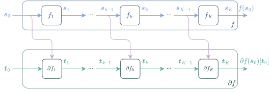
图 8.1：计算链的前向模式自动微分。为便于阅读，我们将中间 JVP 记为关于两个变量

\partial f_{k}:{\bm{s}}_{k-1},{\bm{t}}_{k-1}\mapsto\partial f_{k}({\bm{s}}_{k-1})[{\bm{t}}_{k-1}]

与

\partial f_{k}({\bm{s}}_{k-1})[{\bm{t}}_{k-1}]={\bm{t}}_{k}

的函数。Figure 8.1: Forward-mode autodiff for a computation chain. For readability, we denoted the intermediate JVP as a function of two variables

\partial f_{k}:{\bm{s}}_{k-1},{\bm{t}}_{k-1}\mapsto\partial f_{k}({\bm{s}}_{k-1})[{\bm{t}}_{k-1}]

with

\partial f_{k}({\bm{s}}_{k-1})[{\bm{t}}_{k-1}]={\bm{t}}_{k}

.

算法 1 计算链的前向模式自动微分Algorithm 1 Forward-mode autodiff for computation chains

1: Functions:

f\coloneqq f_{K}\circ\ldots\circ f_{1}

2: Inputs: input

{\bm{s}}_{0}\in\mathcal{S}_{0}

, input direction

{\bm{v}}\in\mathcal{S}_{0}

3: Initialize

{\bm{t}}_{0}\coloneqq{\bm{v}}

4: for

k\coloneqq 1,\ldots,K

do

5: Compute

{\bm{s}}_{k}\coloneqq f_{k}({\bm{s}}_{k-1})\in\mathcal{S}_{k}

6: Compute

{\bm{t}}_{k}\coloneqq\partial f_{k}({\bm{s}}_{k-1})[{\bm{t}}_{k-1}]\in\mathcal{S}_{k}

7: Outputs:

f({\bm{s}}_{0})\coloneqq{\bm{s}}_{K}

,

\partial f({\bm{s}}_{0})[{\bm{v}}]={\bm{t}}_{K}

计算复杂度Computational complexity

JVP 完全遵循 $f$ 的计算过程，只是额外传播一个变量 ${\bm{t}}_{k}$ 。若认为计算 $\partial f_{k}$ 的代价大致与计算 $f_{k}$ 相当，那么计算一个 JVP 的计算代价大致是 $f$ 的两倍。更一般、更形式化的表述参见 8.3.3 节。The JVP follows exactly the computations of $f$ , with an additional variable ${\bm{t}}_{k}$ being propagated. If we consider that computing $\partial f_{k}$ is roughly as costly as computing $f_{k}$ , then computing a JVP has roughly twice the computational cost of $f$ . See Section 8.3.3 for a more general and more formal statement.

内存占用Memory usage

程序在给定求值步骤的内存占用，是指为确保执行完所有剩余步骤而需要存储在内存中的变量数量。程序的内存代价则是所有求值步骤中内存占用的最大值。就本书的目的而言，我们通过考察给定的程序来分析内存占用与内存代价。关于读、写、删除等内存操作及其相关内存代价的形式化定义，见 [87，第 4 章]。The memory usage of a program at a given evaluation step is the number of variables that need to be stored in memory to ensure the execution of all remaining steps. The memory cost of a program is then the maximal memory usage over all evaluation steps. For our purposes, we analyze the memory usage and memory cost by examining the given program. Formal definitions of operations on memory such as read, write, delete and associated memory costs are presented by [87, Chapter 4].

例如，为了执行链 $f=f_{K}\circ\dots\circ f_{1}$ ，在每一步 $k$ 处，我们只需能够访问 ${\bm{s}}_{k-1}$ ，即可执行程序的其余部分。在计算 ${\bm{s}}_{k}$ 时，我们可以从内存中删除 ${\bm{s}}_{k-1}$ ，并以 ${\bm{s}}_{k}$ 取而代之。因此，与求值 $f$ 相关的内存代价，仅仅是各 ${\bm{s}}_{k}$ 变量的最大维度。For example, to execute the chain $f=f_{K}\circ\dots\circ f_{1}$ , at each step $k$ , we only need to have access to ${\bm{s}}_{k-1}$ to execute the rest of the program. As we compute ${\bm{s}}_{k}$ , we can delete ${\bm{s}}_{k-1}$ from memory and replace it by ${\bm{s}}_{k}$ . Therefore, the memory cost associated with the evaluation of $f$ is just the maximal dimension of the ${\bm{s}}_{k}$ variables.

对于前向模式自动微分，由于我们遵循 $f$ 的计算过程，在每一步 $k$ 处，我们只需能够访问 ${\bm{s}}_{k-1}$ 与 ${\bm{t}}_{k-1}$ ，即可执行程序的其余部分。 ${\bm{s}}_{k-1}$ 与 ${\bm{t}}_{k-1}$ 所占用的内存，一旦 ${\bm{s}}_{k},{\bm{t}}_{k}$ 计算完成，就可以直接用于后者。与 JVP 相关的内存占用总结于图 8.2。总体而言，JVP 的内存代价正好是该函数本身内存代价的两倍。For forward mode autodiff, as we follow the computations of $f$ , at each step $k$ , we only need to have access to ${\bm{s}}_{k-1}$ and ${\bm{t}}_{k-1}$ to execute the rest of the program. The memory used by ${\bm{s}}_{k-1}$ and ${\bm{t}}_{k-1}$ can directly be used for ${\bm{s}}_{k},{\bm{t}}_{k}$ once they are computed. The memory usage associated with the JVP is summarized in Fig. 8.2. Overall the memory cost of the JVP is then exactly twice the memory cost of the function itself.

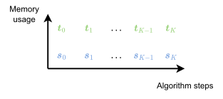
图 8.2：计算链的前向模式自动微分在各步的内存占用。此处

{\bm{t}}_{0}={\bm{v}}

，

{\bm{s}}_{K}=f({\bm{s}}_{0})

，

{\bm{t}}_{K}=\partial f({\bm{s}}_{0})[{\bm{v}}]

。Figure 8.2: Memory usage of forward-mode autodiff for a computation chain. Here

{\bm{t}}_{0}={\bm{v}}

,

{\bm{s}}_{K}=f({\bm{s}}_{0})

,

{\bm{t}}_{K}=\partial f({\bm{s}}_{0})[{\bm{v}}]

.

8.1.2 反向模式Reverse-mode

在机器学习中，我们需要计算梯度的大多数函数都形如 $\ell\circ f$ ，其中 $\ell$ 是标量值损失函数， $f$ 是一个网络。如命题 2.2.13 所示，梯度具有如下形式In machine learning, most functions whose gradient we need to compute take the form $\ell\circ f$ , where $\ell$ is a scalar-valued loss function and $f$ is a network. As seen in Proposition 2.2.13, the gradient takes the form

\nabla(\ell\circ f)({\bm{s}}_{0})=\partial f({\bm{s}}_{0})^{*}[\nabla\ell(f({\bm{s}}_{0}))].

这正是要对 $\nabla\ell(f({\bm{s}}_{0}))\in\mathcal{S}_{K}$ 应用伴随 $\partial f({\bm{s}}_{0})^{*}$ ，并且更一般地对任意输出方向 ${\bm{u}}\in\mathcal{S}_{K}$ 应用伴随的动机所在。由命题 2.3.11 可得This motivates the need for applying the adjoint $\partial f({\bm{s}}_{0})^{*}$ to $\nabla\ell(f({\bm{s}}_{0}))\in\mathcal{S}_{K}$ and more generally to any output direction ${\bm{u}}\in\mathcal{S}_{K}$ . From Proposition 2.3.11, we have

\partial f({\bm{s}}_{0})^{*}=\partial f_{1}({\bm{s}}_{0})^{*}\circ\ldots\circ\partial f_{K}({\bm{s}}_{K-1})^{*}.

在输出方向 ${\bm{u}}\in\mathcal{S}_{K}$ 上对 $\partial f({\bm{s}}_{0})^{*}$ 求值，可分解为Evaluating $\partial f({\bm{s}}_{0})^{*}$ on an output direction ${\bm{u}}\in\mathcal{S}_{K}$ is decomposed as

$\displaystyle{\bm{r}}_{K}$	$\displaystyle\coloneqq{\bm{u}}$
$\displaystyle{\bm{r}}_{K-1}$	$\displaystyle\coloneqq\partial f_{K}({\bm{s}}_{K-1})^{*}[{\bm{r}}_{K}]$
	$\displaystyle\hskip 6.0pt\vdots$
$\displaystyle{\bm{r}}_{0}$	$\displaystyle\coloneqq\partial f_{1}({\bm{s}}_{0})^{*}[{\bm{r}}_{1}]$
$\displaystyle\partial f({\bm{s}}_{0})^{*}[{\bm{u}}]$	$\displaystyle\coloneqq{\bm{r}}_{0}.$

每个中间伴随 $\partial f_{k}({\bm{s}}_{k-1})^{*}$ 都对应一个向量—雅可比乘积（VJP）。它与前向模式的关键区别在于，该过程沿计算链反向进行，反向模式自动微分之名即由此而来。这也可视为对式 8.2 从左向右依次相乘。该过程如图 8.3 所示，并总结于算法 2。Each intermediate adjoint $\partial f_{k}({\bm{s}}_{k-1})^{*}$ amounts to a vector-Jacobian product (VJP). The key difference with the forward mode is that the procedure runs backward through the chain, hence the name reverse mode autodiff. This can also be seen as multiplying Eq. 8.2 from left to right. The procedure is illustrated in Fig. 8.3 and summarized in Algorithm 2.

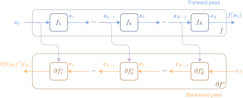
图 8.3：计算链的反向模式自动微分。为便于阅读，我们将中间 VJP 记作二元函数

\partial f_{k}^{*}:({\bm{s}}_{k-1},{\bm{r}}_{k})\mapsto\partial f_{k}({\bm{s}}_{k-1})^{*}[{\bm{r}}_{k}]

，其中

\partial f_{k}({\bm{s}}_{k-1})^{*}[{\bm{r}}_{k}]={\bm{r}}_{k-1}

。Figure 8.3: Reverse mode of automatic differentiation for a computation chain. For readability, we denoted the intermediate VJPs as functions of two variables

\partial f_{k}^{*}:({\bm{s}}_{k-1},{\bm{r}}_{k})\mapsto\partial f_{k}({\bm{s}}_{k-1})^{*}[{\bm{r}}_{k}]

, with

\partial f_{k}({\bm{s}}_{k-1})^{*}[{\bm{r}}_{k}]={\bm{r}}_{k-1}

.

算法 2 计算链的反向模式自动微分Algorithm 2 Reverse-mode autodiff for computation chains

1: Functions:

f\coloneqq f_{K}\circ\ldots\circ f_{1}

,

2: Inputs: input

{\bm{s}}_{0}\in\mathcal{S}_{0}

, output direction

{\bm{u}}\in\mathcal{S}_{K}

3: for

k\coloneqq 1,\ldots,K

do

\triangleright

Forward pass

4: Compute

{\bm{s}}_{k}\coloneqq f_{k}({\bm{s}}_{k-1})\in\mathcal{S}_{k}

5: Initialize

{\bm{r}}_{K}\coloneqq{\bm{u}}

.

6: for

k\coloneqq K,\ldots,1

do

\triangleright

Backward pass

7: Compute

{\bm{r}}_{k-1}\coloneqq\partial f_{k}({\bm{s}}_{k-1})^{*}[{\bm{r}}_{k}]\in\mathcal{S}_{k-1}

8: Outputs:

f({\bm{s}}_{0})\coloneqq{\bm{s}}_{K}

,

\partial f({\bm{s}}_{0})^{*}[{\bm{u}}]={\bm{r}}_{0}

计算复杂性Computational complexity

就运算次数而言，VJP 不过两次经过计算链：一次前向，一次反向。若认为中间 VJP 的代价与中间函数本身大致相当，则 VJP 的代价恰好是原函数代价的两倍，与 JVP 相同。更一般、更形式化的陈述见 8.3.3 节。In terms of number of operations, the VJP simply passes two times through the chain, once forward, then backward. If we consider the intermediate VJPs to be roughly as costly as the intermediate functions themselves, the VJP amounts to just twice the cost of the original function, just as the JVP. See Section 8.3.3 for a more generic and formal statement.

内存占用Memory usage

回想一下，程序在给定求值步骤的内存占用，是指为确保执行完剩余步骤而需存储在内存中的变量数量。考察算法 3，为执行所有反向步骤，即第 6 行的循环，我们需要能够访问全部中间输入 ${\bm{s}}_{0},\ldots,{\bm{s}}_{K-1}$ 。因此，反向模式自动微分的内存代价与计算链的长度 $K$ 成正比。图 8.4 展示了反向模式自动微分过程中的内存占用：它线性增长，直至前向传播结束，随后逐渐下降，直至输出函数值与 VJP。这一内存代价可借助 8.5 节介绍的检查点技术加以缓解。Recall that the memory usage of a program at a given evaluation step is the number of variables that need to be stored in memory to ensure the execution of the remaining steps. If we inspect Algorithm 3, to execute all backward steps, that is the loop in line 6, we need to have access to all the intermediate inputs ${\bm{s}}_{0},\ldots,{\bm{s}}_{K-1}$ . Therefore, the memory cost of reverse-mode autodiff is proportional to the length of the chain $K$ . Fig. 8.4 illustrates the memory usage during reverse mode autodiff. It grows linearly until the end of the forward pass and then progressively decreases until it outputs the value of the function and the VJP. The memory cost can be mitigated by means of checkpointing techniques presented in Section 8.5.

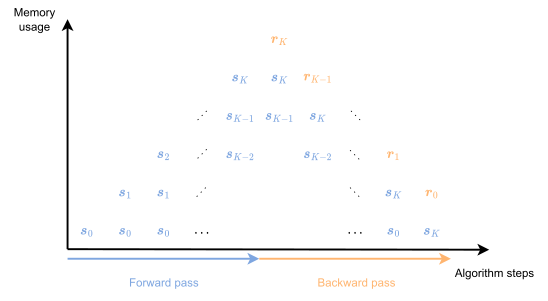
图 8.4：计算链的反向模式自动微分的内存占用。Figure 8.4: Memory usage of reverse mode autodiff for a computation chain.

函数求值与 VJP 求值相解耦Decoupled function and VJP evaluations

反向模式自动微分额外的内存开销也带来了一些优势。若我们需要对 $n$ 个不同的输出方向 ${\bm{u}}_{i}$ 计算 $\partial f({\bm{s}}_{0})^{*}[{\bm{u}}_{i}]$ ，只须计算并存储一次中间计算 ${\bm{s}}_{k}$ ，再对反向传播进行 $n$ 次调用即可。换言之，将中间计算 ${\bm{s}}_{k}$ 存入内存，我们便可实例化一个 VJP 算子，并通过反向传播将其作用于任意 ${\bm{u}}$ 。形式上，前向传播与反向传播可以解耦为The additional memory cost of reverse mode autodiff comes with some advantages. If we need to compute $\partial f({\bm{s}}_{0})^{*}[{\bm{u}}_{i}]$ for $n$ different output directions ${\bm{u}}_{i}$ , we only need to compute and store once the intermediate computations ${\bm{s}}_{k}$ and then make $n$ calls to the backward pass. In other words, by storing in memory the intermediate computations ${\bm{s}}_{k}$ , we may instantiate a VJP operator, which we may apply to any ${\bm{u}}$ through the backward pass. Formally, the forward and backward passes can be decoupled as

\mathrm{forward}(f,{\bm{s}}_{0})\coloneqq(f({\bm{s}}_{0}),\partial f({\bm{s}}_{0})^{*})

其中where

\partial f({\bm{s}}_{0})^{*}[{\bm{u}}]\coloneqq\mathrm{backward}({\bm{u}};{\bm{s}}_{0},\ldots,{\bm{s}}_{K-1}).

在函数式编程的术语中，VJP $\partial f({\bm{s}}_{0})^{*}$ 是一个闭包，因为它包含了中间计算结果 ${\bm{s}}_{0},\dots,{\bm{s}}_{K-1}$ 。若要将其用于多个方向 ${\bm{v}}_{i}$ ，JVP $\partial f({\bm{s}}_{0})$ 亦可同样处理。In functional programming terminology, the VJP $\partial f({\bm{s}}_{0})^{*}$ is a closure, as it contains the intermediate computations ${\bm{s}}_{0},\dots,{\bm{s}}_{K-1}$ . The same can be done for the JVP $\partial f({\bm{s}}_{0})$ if we want to apply it to multiple directions ${\bm{v}}_{i}$ .

例 8.1.1（参数固定的多层感知机）。Example 8.1.1 (Multilayer perceptron with fixed parameters ).

作为一个贯穿全章的示例，考虑具有一个隐藏层且（目前）给定固定权重的多层感知机（MLP）。如第 4 章所述，MLP 可分解为As a running example, consider a multilayer perceptron (MLP) with one hidden layer and (for now) given fixed weights. As presented in Chapter 4, an MLP can be decomposed as

\displaystyle{\bm{s}}_{0}

\displaystyle={\bm{x}}

\displaystyle{\bm{s}}_{1}

\displaystyle=f_{1}({\bm{s}}_{0})=\sigma({\bm{A}}_{1}{\bm{s}}_{0}+{\bm{b}}_{1})

\displaystyle{\bm{s}}_{2}

\displaystyle=f_{2}({\bm{s}}_{1})={\bm{A}}_{2}{\bm{s}}_{1}+{\bm{b}}_{2}

\displaystyle f({\bm{x}})

\displaystyle={\bm{s}}_{2},

其中

{\bm{A}}_{1},{\bm{A}}_{2},{\bm{b}}_{1},{\bm{b}}_{2}

为某些固定参数，

\sigma

为激活函数，例如 softplus 激活函数

\sigma(x)=\log(1+e^{x})

，其导数为

\sigma^{\prime}(x)=e^{x}/(1+e^{x})

。for

{\bm{A}}_{1},{\bm{A}}_{2},{\bm{b}}_{1},{\bm{b}}_{2}

some fixed parameters and

\sigma

an activation function such as the softplus activation function

\sigma(x)=\log(1+e^{x})

with derivative

\sigma^{\prime}(x)=e^{x}/(1+e^{x})

. 于是，

f

在输入

{\bm{x}}

上沿方向

{\bm{v}}

的 JVP 可分解为Evaluating the JVP of

f

on an input

{\bm{x}}

along a direction

{\bm{v}}

can then be decomposed as

\displaystyle{\bm{t}}_{0}

\displaystyle={\bm{v}}

\displaystyle{\bm{t}}_{1}

\displaystyle=\sigma^{\prime}({\bm{A}}_{1}{\bm{s}}_{0}+{\bm{b}}_{1})\odot({\bm{A}}_{1}{\bm{t}}_{0})

\displaystyle{\bm{t}}_{2}

\displaystyle={\bm{A}}_{2}{\bm{t}}_{1}

\displaystyle\partial f({\bm{x}})[{\bm{v}}]

\displaystyle={\bm{t}}_{2},

其中第二行我们使用了例 8.4.2 中逐元素函数的 JVP。where we used in the second line the JVP of element-wise functions as in Example 8.4.2. 在

{\bm{x}}

处计算

f

的 VJP，需要在已存储的激活值处计算各中间 VJPEvaluating the VJP of

f

at

{\bm{x}}

requires evaluating the intermediate VJPs at the stored activations

\displaystyle{\bm{r}}_{2}

\displaystyle={\bm{u}}

\displaystyle{\bm{r}}_{1}

\displaystyle=\partial f_{2}({\bm{s}}_{1})^{*}[{\bm{r}}_{2}]={\bm{A}}_{2}^{\top}{\bm{r}}_{2}

\displaystyle{\bm{r}}_{0}

\displaystyle=\partial f_{1}({\bm{s}}_{0})^{*}[{\bm{r}}_{1}]={\bm{A}}_{1}^{\top}(\sigma^{\prime}({\bm{A}}_{1}{\bm{s}}_{0}+{\bm{b}}_{1})\odot{\bm{r}}_{1})

\displaystyle\partial f({\bm{x}})^{*}[{\bm{u}}]

\displaystyle={\bm{r}}_{0}.

8.1.3 计算完整雅可比矩阵的复杂度Complexity of computing entire Jacobians

本节分析前向模式与反向模式自动微分在计算计算链 $f=f_{K}\circ\dots\circ f_{1}$ 的完整雅可比矩阵 $\bm{\partial}f({\bm{s}}_{0})$ 时所需的时间与空间复杂度，其中 $f_{k}\colon\mathcal{S}_{k-1}\to\mathcal{S}_{k}$ 。我们假设 $\mathcal{S}_{k}\subseteq\mathbb{R}^{D_{k}}$ 、 $D_{K}=M$ 与 $D_{0}=D$ 。于是有 $f\colon\mathbb{R}^{D}\to\mathbb{R}^{M}$ 与 $\bm{\partial}f({\bm{s}}_{0})\in\mathbb{R}^{M\times D}$ 。In this section, we analyze the time and space complexities of forward-mode and reverse-mode autodiff for computing the entire Jacobian matrix $\bm{\partial}f({\bm{s}}_{0})$ of a computation chain $f=f_{K}\circ\dots\circ f_{1}$ , where $f_{k}\colon\mathcal{S}_{k-1}\to\mathcal{S}_{k}$ . We assume $\mathcal{S}_{k}\subseteq\mathbb{R}^{D_{k}}$ , $D_{K}=M$ and $D_{0}=D$ . Therefore, we have $f\colon\mathbb{R}^{D}\to\mathbb{R}^{M}$ and $\bm{\partial}f({\bm{s}}_{0})\in\mathbb{R}^{M\times D}$ .

前向模式自动微分的复杂度Complexity of forward-mode autodiff

根据定义 2.2.8，对每个 $j\in[D]$ ，将雅可比矩阵与标准基向量 ${\bm{e}}_{j}\in\mathbb{R}^{D}$ 相乘，即可提取出该矩阵的第 $[\bm{\partial}f({\bm{s}}_{0})]_{:,j}\in\mathbb{R}^{M}$ 列：Using Definition 2.2.8, we find that we can extract each column $[\bm{\partial}f({\bm{s}}_{0})]_{:,j}\in\mathbb{R}^{M}$ of the Jacobian matrix, for $j\in[D]$ , by multiplying with the standard basis vector ${\bm{e}}_{j}\in\mathbb{R}^{D}$ :

$\displaystyle[\bm{\partial}f({\bm{s}}_{0})]_{:,1}$	$\displaystyle=\partial f({\bm{s}}_{0})[{\bm{e}}_{1}]$

$\displaystyle[\bm{\partial}f({\bm{s}}_{0})]_{:,D}$	$\displaystyle=\partial f({\bm{s}}_{0})[{\bm{e}}_{D}].$

因此，计算完整雅可比矩阵所需的 JVP 个数为 $D$ ，且所用向量取自 $\mathbb{R}^{D}$ 。设链式组合中的每个 $f_{k}$ 均具有形式 $f_{k}:\mathbb{R}^{D_{k-1}}\rightarrow\mathbb{R}^{D_{k}}$ ，若将其视为矩阵，则 $\bm{\partial}f_{k}({\bm{s}}_{k-1})$ 的大小为 $D_{k}\times D_{k-1}$ 。于是， $D$ 个 JVP 的计算代价为 $O\left(D\sum_{k=1}^{K}D_{k}D_{k-1}\right)$ 。由于每处理完一层即可释放其对应的中间计算，内存代价为 $O(\max_{k\in[K]}D_{k})$ 。为简单起见设 $D_{1}=\dots=D_{K-1}=D$ ，并利用 $D_{K}=M$ ，可知计算 $D$ 个 JVP 的计算代价——也就是以前向模式自动微分计算完整雅可比矩阵的代价——为 $O(MD^{2}+KD^{3})$ ，内存代价为 $O(\max\{D,M\})$ 。若函数只有一个输入（ $D=1$ ），前向模式可一次算出整个雅可比矩阵，此时问题归结为单个方向导数。Computing the full Jacobian matrix therefore requires $D$ JVPs with vectors in $\mathbb{R}^{D}$ . Assuming each $f_{k}$ in the chain composition has the form $f_{k}:\mathbb{R}^{D_{k-1}}\rightarrow\mathbb{R}^{D_{k}}$ , seen as a matrix, $\bm{\partial}f_{k}({\bm{s}}_{k-1})$ has size $D_{k}\times D_{k-1}$ . Therefore, the computational cost of $D$ JVPs is $O\left(D\sum_{k=1}^{K}D_{k}D_{k-1}\right)$ . The memory cost is $O(\max_{k\in[K]}D_{k})$ , since we can release intermediate computations after each layer is processed. Setting $D_{1}=\dots=D_{K-1}=D$ for simplicity and using $D_{K}=M$ , we obtain that the computational cost of computing $D$ JVPs and therefore of computing the full Jacobian matrix by forward-mode autodiff is $O(MD^{2}+KD^{3})$ . The memory cost is $O(\max\{D,M\})$ . If a function has a single input ( $D=1$ ), then the forward mode computes the entire Jacobian at once, which reduces to a single directional derivative.

反向模式自动微分的复杂度Complexity of reverse-mode autodiff

根据定义 2.2.8，对每个 $i\in[M]$ ，将雅可比矩阵 $[\bm{\partial}f({\bm{s}}_{0})]_{i}\in\mathbb{R}^{D}$ 与标准基向量 ${\bm{e}}_{i}\in\mathbb{R}^{M}$ 相乘，即可提取出该矩阵的每一行：Using Definition 2.2.8, we find that we can extract each row of the Jacobian matrix $[\bm{\partial}f({\bm{s}}_{0})]_{i}\in\mathbb{R}^{D}$ , for $i\in[M]$ , by multiplying with the standard basis vector ${\bm{e}}_{i}\in\mathbb{R}^{M}$ :

$\displaystyle[\bm{\partial}f({\bm{s}}_{0})]_{1}$	$\displaystyle=\partial f({\bm{s}}_{0})^{*}[{\bm{e}}_{1}]$

$\displaystyle[\bm{\partial}f({\bm{s}}_{0})]_{M}$	$\displaystyle=\partial f({\bm{s}}_{0})^{*}[{\bm{e}}_{M}].$

因此，计算完整雅可比矩阵需要执行 $M$ 次 VJP，所用向量取自 $\mathbb{R}^{M}$ 。按前述假设，链式组合中的每个 $f_{k}$ 均具有形式 $f_{k}:\mathbb{R}^{D_{k-1}}\rightarrow\mathbb{R}^{D_{k}}$ ，于是 $M$ 次 VJP 的计算代价为 $O\left(M\sum_{k=1}^{K}D_{k}D_{k-1}\right)$ 。然而，内存代价为 $O(\sum_{k=1}^{K}D_{k})$ ，因为我们需要为 $K$ 层中的每一层存储中间计算结果。为简单起见，设 $D_{0}=\dots=D_{K-1}=D$ ，并利用 $D_{K}=M$ ，可得计算 $M$ 次 VJP 的计算代价，亦即用反向模式自动微分计算完整雅可比矩阵的代价，为 $O(M^{2}D+KMD^{2})$ ；内存代价则为 $O(KD+M)$ 。若函数只有一个输出（ $M=1$ ），反向模式自动微分便可一次算出整个雅可比矩阵，此时问题归结为计算梯度。Computing the full Jacobian matrix therefore requires $M$ VJPs with vectors in $\mathbb{R}^{M}$ . Assuming as before that each $f_{k}$ in the chain composition has the form $f_{k}:\mathbb{R}^{D_{k-1}}\rightarrow\mathbb{R}^{D_{k}}$ , the computational cost of $M$ VJPs is $O\left(M\sum_{k=1}^{K}D_{k}D_{k-1}\right)$ . However, the memory cost is $O(\sum_{k=1}^{K}D_{k})$ , as we need to store the intermediate computations for each of the $K$ layers. Setting $D_{0}=\dots=D_{K-1}=D$ for simplicity and using $D_{K}=M$ , we obtain that the computational cost of computing $M$ VJPs and therefore of computing the full Jacobian matrix by reverse-mode autodiff is $O(M^{2}D+KMD^{2})$ . The memory cost is $O(KD+M)$ . If the function has a single output ( $M=1$ ), reverse-mode autodiff computes the entire Jacobian at once, which reduces to the gradient.

何时应当使用前向模式自动微分，何时又该使用反向模式自动微分？When to use forward-mode vs. reverse-mode autodiff?

我们在表 8.1 中总结时间与空间复杂度。一般而言，若 $M<D$ ，则反向模式更具优势，代价是要占用一些内存；若 $M\geq D$ ，则前向模式更具优势。We summarize the time and space complexities in Table 8.1. Generally, if $M<D$ , reverse-mode is more advantageous at the price of some memory cost. If $M\geq D$ , forward mode is more advantageous.

	前向模式Forward-mode	反向模式Reverse-mode
时间Time	$O(MD^{2}+KD^{3})$	$O(M^{2}D+KMD^{2})$
空间Space	$O(\max\{M,D\})$	$O(KD+M)$

表 8.1：计算函数链

f=f_{K}\circ\dots\circ f_{1}

的完整雅可比矩阵时，前向模式与反向模式自动微分的时间与空间复杂度，其中当

k=1,\dots,K-1

时

f_{k}\colon\mathbb{R}^{D}\to\mathbb{R}^{D}

，且

f_{K}\colon\mathbb{R}^{D}\to\mathbb{R}^{M}

。我们假设每个

\partial f_{k}

均为稠密线性算子。前向模式需要

D

次 JVP，反向模式需要

M

次 VJP。Table 8.1: Time and space complexities of forward-mode and reverse-mode autodiff for computing the full Jacobian of a chain of functions

f=f_{K}\circ\dots\circ f_{1}

, where

f_{k}\colon\mathbb{R}^{D}\to\mathbb{R}^{D}

if

k=1,\dots,K-1

and

f_{K}\colon\mathbb{R}^{D}\to\mathbb{R}^{M}

. We assume

\partial f_{k}

is a dense linear operator. Forward mode requires

D

JVPs. Reverse mode requires

M

VJPs.

8.2 前馈网络8.2 Feedforward networks

上一节中，我们针对输入为 ${\bm{s}}_{0}\in\mathcal{S}_{0}$ 的计算链推导了前向模式自动微分与反向模式自动微分。本节中，我们转而推导前馈网络的反向模式自动微分；此时每一层 $f_{k}$ 都允许显式依赖于一些额外参数 ${\bm{w}}_{k}\in\mathcal{W}_{k}$ 。其递推关系为In the previous section, we derived forward-mode autodiff and reverse-mode autodiff for computation chains with an input ${\bm{s}}_{0}\in\mathcal{S}_{0}$ . In this section, we now derive reverse-mode autodiff for feedforward networks, in which each layer $f_{k}$ is now allowed to depend explicitly on some additional parameters ${\bm{w}}_{k}\in\mathcal{W}_{k}$ . The recursion is

$\displaystyle{\bm{s}}_{0}$	$\displaystyle\coloneqq{\bm{x}}\in\mathcal{S}_{0}$
$\displaystyle{\bm{s}}_{1}$	$\displaystyle\coloneqq f_{1}({\bm{s}}_{0},{\bm{w}}_{1})\in\mathcal{S}_{1}$
	$\displaystyle\hskip 6.0pt\vdots$
$\displaystyle{\bm{s}}_{K}$	$\displaystyle\coloneqq f_{K}({\bm{s}}_{K-1},{\bm{w}}_{K})\in\mathcal{S}_{K}$
$\displaystyle f({\bm{x}},{\bm{w}})$	$\displaystyle\coloneqq{\bm{s}}_{K},$

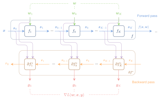
其中 $\mathcal{S}_{0}=\mathcal{X}$ ，且 ${\bm{w}}=({\bm{w}}_{1},\dots,{\bm{w}}_{K})\in\mathcal{W}_{1}\times\dots\times\mathcal{W}_{K}$ 。每个 $f_{k}$ 现在都是两个自变量的函数：第一个自变量依赖于前一层，第二个自变量则不然。图 8.5 对此作了图示。下面说明如何对前馈网络求导。where $\mathcal{S}_{0}=\mathcal{X}$ and ${\bm{w}}=({\bm{w}}_{1},\dots,{\bm{w}}_{K})\in\mathcal{W}_{1}\times\dots\times\mathcal{W}_{K}$ . Each $f_{k}$ is now a function of two arguments. The first argument depends on the previous layer, but the second argument does not. This is illustrated in Fig. 8.5. We now explain how to differentiate a feedforward network.

8.2.1 计算伴随Computing the adjoint

该函数的形式为 $f\colon\mathcal{E}\to\mathcal{F}$ ，其中 $\mathcal{E}\coloneqq\mathcal{X}\times(\mathcal{W}_{1}\times\dots\times\mathcal{W}_{K})$ 、 $\mathcal{F}\coloneqq\mathcal{S}_{K}$ 。由 2.3 节可知，VJP 的形式为 $\partial f({\bm{x}},{\bm{w}})^{*}\colon\mathcal{F}\to\mathcal{E}$ 。因此，我们希望做到：对任意 ${\bm{u}}\in\mathcal{F}$ ，都能计算 $\partial f({\bm{x}},{\bm{w}})^{*}[{\bm{u}}]\in\mathcal{E}$ 。The function has the form $f\colon\mathcal{E}\to\mathcal{F}$ , where $\mathcal{E}\coloneqq\mathcal{X}\times(\mathcal{W}_{1}\times\dots\times\mathcal{W}_{K})$ and $\mathcal{F}\coloneqq\mathcal{S}_{K}$ . From Section 2.3, we know that the VJP has the form $\partial f({\bm{x}},{\bm{w}})^{*}\colon\mathcal{F}\to\mathcal{E}$ . Therefore, we want to be able to compute $\partial f({\bm{x}},{\bm{w}})^{*}[{\bm{u}}]\in\mathcal{E}$ for any ${\bm{u}}\in\mathcal{F}$ .

好在反向递推只需对计算链的情形稍加修改。事实上，由于 $f_{k}\colon\mathcal{E}_{k}\to\mathcal{F}_{k}$ ，其中 $\mathcal{E}_{k}\coloneqq\mathcal{S}_{k-1}\times\mathcal{W}_{k}$ 、 $\mathcal{F}_{k}\coloneqq\mathcal{S}_{k}$ ，故中间 VJP 的形式为 $\partial f_{k}({\bm{s}}_{k-1},{\bm{w}}_{k})^{*}\colon\mathcal{F}_{k}\to\mathcal{E}_{k}$ 。由此得到递推式Fortunately, the backward recursion is only a slight modification of the computation chain case. Indeed, since $f_{k}\colon\mathcal{E}_{k}\to\mathcal{F}_{k}$ , where $\mathcal{E}_{k}\coloneqq\mathcal{S}_{k-1}\times\mathcal{W}_{k}$ and $\mathcal{F}_{k}\coloneqq\mathcal{S}_{k}$ , the intermediate VJPs have the form $\partial f_{k}({\bm{s}}_{k-1},{\bm{w}}_{k})^{*}\colon\mathcal{F}_{k}\to\mathcal{E}_{k}$ . We therefore arrive at the recursion

$\displaystyle{\bm{r}}_{K}$	$\displaystyle={\bm{u}}\in\mathcal{S}_{K}$
$\displaystyle({\bm{r}}_{K-1},{\bm{g}}_{K})$	$\displaystyle=\partial f_{K}({\bm{s}}_{K-1},{\bm{w}}_{K})^{*}[{\bm{r}}_{K}]\in\mathcal{S}_{K-1}\times\mathcal{W}_{K}$
	$\displaystyle\hskip 6.0pt\vdots$
$\displaystyle({\bm{r}}_{0},{\bm{g}}_{1})$	$\displaystyle=\partial f_{1}({\bm{s}}_{0},{\bm{w}}_{1})^{*}[{\bm{r}}_{1}]\in\mathcal{S}_{0}\times\mathcal{W}_{1}.$

最终输出为The final output is

\partial f({\bm{x}},{\bm{w}})^{*}[{\bm{u}}]=({\bm{r}}_{0},({\bm{g}}_{1},\dots,{\bm{g}}_{K})).

8.2.2 计算梯度Computing the gradient

我们常常把网络与一个损失函数复合起来We often compose a network with a loss function

L({\bm{w}};{\bm{x}},{\bm{y}})\coloneqq\ell(f({\bm{x}},{\bm{w}});{\bm{y}})\in\mathbb{R}.

由命题 2.3.11，梯度由下式给出From Proposition 2.3.11, the gradient is given by

\nabla L({\bm{w}};{\bm{x}},{\bm{y}})=({\bm{g}}_{1},\dots,{\bm{g}}_{K})\in\mathcal{W}_{1}\times\dots\times\mathcal{W}_{K}

其中where

\partial f({\bm{x}},{\bm{w}})^{*}[{\bm{u}}]=({\bm{r}}_{0},({\bm{g}}_{1},\dots,{\bm{g}}_{K})),

且 ${\bm{u}}=\nabla\ell(f({\bm{x}},{\bm{w}});{\bm{y}})\in\mathcal{S}_{K}$ 。输出 ${\bm{r}}_{0}\in\mathcal{S}_{0}$ （其中 $\mathcal{S}_{0}=\mathcal{X}$ ）对应于关于 ${\bm{x}}\in\mathcal{X}$ 的梯度，通常并不需要，只有生成建模场合才会用到。完整流程总结于算法 3。with ${\bm{u}}=\nabla\ell(f({\bm{x}},{\bm{w}});{\bm{y}})\in\mathcal{S}_{K}$ . The output ${\bm{r}}_{0}\in\mathcal{S}_{0}$ , where $\mathcal{S}_{0}=\mathcal{X}$ , corresponds to the gradient w.r.t. ${\bm{x}}\in\mathcal{X}$ and is typically not needed, except in generative modeling settings. The full procedure is summarized in Algorithm 3.

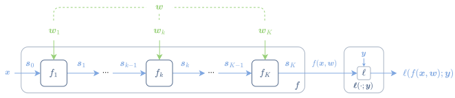
图 8.5：将 MLP 视为其参数的函数时的计算图。Figure 8.5: Computation graph of an MLP as a function of its parameters.

图 8.6：自动微分的反向模式，又称梯度反向传播，用于计算 MLP 在给定一个输入—标签对时的损失梯度。为便于阅读，我们把中间 VJP 写成三个变量的函数

\partial f_{k}^{*}:({\bm{s}}_{k-1},{\bm{w}}_{k-1},{\bm{r}}_{k})\mapsto\partial f_{k}({\bm{s}}_{k-1},{\bm{w}}_{k})^{*}[{\bm{r}}_{k}]

，其中

\partial f_{k}({\bm{s}}_{k-1},{\bm{w}}_{k})^{*}[{\bm{r}}_{k}]=({\bm{r}}_{k-1},{\bm{g}}_{k})

。Figure 8.6: Reverse mode of automatic differentiation, a.k.a., gradient back-propagation to compute the gradient of the loss of an MLP on an input label pair. For readability, we denoted the intermediate VJPs as functions of three variables

\partial f_{k}^{*}:({\bm{s}}_{k-1},{\bm{w}}_{k-1},{\bm{r}}_{k})\mapsto\partial f_{k}({\bm{s}}_{k-1},{\bm{w}}_{k})^{*}[{\bm{r}}_{k}]

with

\partial f_{k}({\bm{s}}_{k-1},{\bm{w}}_{k})^{*}[{\bm{r}}_{k}]=({\bm{r}}_{k-1},{\bm{g}}_{k})

.

算法 3 前馈网络的梯度反向传播Algorithm 3 Gradient back-propagation for feedforward networks

1: Functions:

f_{1},\dots,f_{K}

in sequential order

2: Inputs: data point

({\bm{x}},{\bm{y}})\in\mathcal{X}\times\mathcal{Y}

3: parameters

{\bm{w}}=({\bm{w}}_{1},\ldots,{\bm{w}}_{K})\in\mathcal{W}_{1}\times\dots\times\mathcal{W}_{K}

4: Initialize

{\bm{s}}_{0}\coloneqq{\bm{x}}

\triangleright

Forward pass

5: for

k\coloneqq 1,\ldots,K

do

6: Compute and store

{\bm{s}}_{k}\coloneqq f_{k}({\bm{s}}_{k-1},{\bm{w}}_{k})\in\mathcal{S}_{k}

7: Compute

\ell({\bm{s}}_{K};{\bm{y}})

and

{\bm{u}}\coloneqq\nabla\ell({\bm{s}}_{K};{\bm{y}})\in\mathcal{S}_{K}

8: Initialize

{\bm{r}}_{K}\coloneqq{\bm{u}}\in\mathcal{S}_{K}

\triangleright

Backward pass

9: for

k\coloneqq K,\ldots,1

do

10: Compute

({\bm{r}}_{k-1},{\bm{g}}_{k})\coloneqq\partial f_{k}({\bm{s}}_{k-1},{\bm{w}}_{k})^{*}[{\bm{r}}_{k}]\in\mathcal{S}_{k-1}\times\mathcal{W}_{k}

11: Outputs:

L({\bm{w}};{\bm{x}},{\bm{y}})\coloneqq\ell({\bm{s}}_{K};{\bm{y}})

,

\nabla L({\bm{w}};{\bm{x}},{\bm{y}})=({\bm{g}}_{1},\ldots,{\bm{g}}_{K})

8.3 计算图8.3 Computation graphs

前几节回顾了计算链的自动微分及其向前馈网络的推广。本节回顾它在计算图上的推广，该推广已于 4.1.3 节引入。不失一般性，我们的形式化假设函数可以有多个输入，但只产生单个输出，因为总能把多个输出归并成一个元组。这样一来，输出变量 ${\bm{s}}_{k}$ 与函数 $f_{k}$ 便一一对应。In the previous sections, we reviewed autodiff for computation chains and its extension to feedforward networks. In this section, we review its generalization to computation graphs, introduced in Section 4.1.3. Our formalism assumes, without loss of generality, that functions can take multiple inputs but only produce a single output, as we can always group multiple outputs as a tuple. This enables a one-to-one correspondence between output variables ${\bm{s}}_{k}$ and functions $f_{k}$ .

8.3.1 前向模式Forward mode

前向模式即沿输入方向 ${\bm{v}}\in\mathcal{S}_{0}$ 计算程序的 JVP。对于计算链 $f\coloneqq f_{K}\circ\dots\circ f_{1}$ ，每个 $f_{k}$ 接受单个输入 ${\bm{s}}_{k-1}\in\mathcal{S}_{k-1}$ ，每个 $\partial f_{k}({\bm{s}}_{k-1})$ 接受单个输入方向 ${\bm{t}}_{k-1}\in\mathcal{S}_{k-1}$ 。于是，从 ${\bm{t}}_{0}\coloneqq{\bm{v}}$ 出发，第 $k\in[K]$ 次迭代的前向传播为The forward mode corresponds to computing the JVP of the program in an input direction ${\bm{v}}\in\mathcal{S}_{0}$ . In the case of a computation chain $f\coloneqq f_{K}\circ\dots\circ f_{1}$ , each $f_{k}$ takes a single input ${\bm{s}}_{k-1}\in\mathcal{S}_{k-1}$ and each $\partial f_{k}({\bm{s}}_{k-1})$ takes a single input direction ${\bm{t}}_{k-1}\in\mathcal{S}_{k-1}$ . The forward pass on iteration $k\in[K]$ is then, starting from ${\bm{t}}_{0}\coloneqq{\bm{v}}$ ,

$\displaystyle{\bm{s}}_{k}$	$\displaystyle\coloneqq f_{k}({\bm{s}}_{k-1})\in\mathcal{S}_{k}$
$\displaystyle{\bm{t}}_{k}$	$\displaystyle\coloneqq\partial f_{k}({\bm{s}}_{k-1})[{\bm{t}}_{k-1}]\in\mathcal{S}_{k}.$

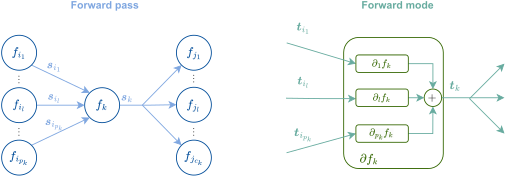
对于由函数 $f_{1},\dots,f_{K}$ 按拓扑序给出的计算图，此时每个 $f_{k}$ 都可以接受多个输入 $({\bm{s}}_{i_{1}},\dots,{\bm{s}}_{i_{p_{k}}})\in\mathcal{S}_{i_{1}}\times\dots\times\mathcal{S}_{i_{p_{k}}}$ ，而每个 $\partial f_{k}({\bm{s}}_{i_{1}},\dots,{\bm{s}}_{i_{p_{k}}})$ 所接受的输入方向 $({\bm{t}}_{i_{1}},\dots,{\bm{t}}_{i_{p_{k}}})\in\mathcal{S}_{i_{1}}\times\dots\times\mathcal{S}_{i_{p_{k}}}$ 也与之数量相同，其中 $(i_{1},\ldots,i_{p_{k}})\coloneqq{\operatorname{pa}}(k)$ 是 $f_{k}$ 的父节点。于是，第 $k\in[K]$ 步的前向传播会同时算出中间输入与中间方向：In the case of a computation graph, specified by functions $f_{1},\dots,f_{K}$ in topological order, each $f_{k}$ may now take multiple inputs $({\bm{s}}_{i_{1}},\dots,{\bm{s}}_{i_{p_{k}}})\in\mathcal{S}_{i_{1}}\times\dots\times\mathcal{S}_{i_{p_{k}}}$ , and each $\partial f_{k}({\bm{s}}_{i_{1}},\dots,{\bm{s}}_{i_{p_{k}}})$ takes as many input directions $({\bm{t}}_{i_{1}},\dots,{\bm{t}}_{i_{p_{k}}})\in\mathcal{S}_{i_{1}}\times\dots\times\mathcal{S}_{i_{p_{k}}}$ , where $(i_{1},\ldots,i_{p_{k}})\coloneqq{\operatorname{pa}}(k)$ are the parents of $f_{k}$ . The forward pass on step $k\in[K]$ then computes both intermediate inputs and directions as

$\displaystyle{\bm{s}}_{k}$	$\displaystyle\coloneqq f_{k}({\bm{s}}_{i_{1}},\dots,{\bm{s}}_{i_{p_{k}}})\in\mathcal{S}_{k}$
$\displaystyle{\bm{t}}_{k}$	$\displaystyle\coloneqq\partial f_{k}({\bm{s}}_{i_{1}},\dots,{\bm{s}}_{i_{p_{k}}})[{\bm{t}}_{i_{1}},\dots,{\bm{t}}_{i_{p_{k}}}]\in\mathcal{S}_{k}.$

回顾一下， $\partial_{i}f_{k}$ 表示对 $f_{k}$ 关于其第 $i$ 个自变量求导。借助命题 2.3.12 中的扇入法则可得，导数按如下方式传播：Let us recall that $\partial_{i}f_{k}$ means that we differentiate $f_{k}$ w.r.t. its $i$ ^th argument. Using the fan-in rule in Proposition 2.3.12, we obtain that the derivatives are propagated as

{\bm{t}}_{k}=\sum_{j=1}^{p_{k}}\partial_{j}f_{k}({\bm{s}}_{i_{1}},\dots,{\bm{s}}_{i_{p_{k}}})[{\bm{t}}_{i_{j}}]\in\mathcal{S}_{k}.

最终输出为 $\partial f({\bm{s}}_{0})[{\bm{v}}]={\bm{t}}_{K}$ 。由此得到的通用前向模式流程总结于图 8.7 与算法 4。直观地说，该算法就是在前向传播过程中逐个计算并累加中间 JVP。尽管文中并未明言，但当没有子节点再依赖节点 $k$ 时，我们便可将 ${\bm{s}}_{k}$ 与 ${\bm{t}}_{k}$ 从内存中释放。The final output is $\partial f({\bm{s}}_{0})[{\bm{v}}]={\bm{t}}_{K}$ . The resulting generic forward-mode procedure is summarized in Fig. 8.7 and in Algorithm 4. Intuitively, the algorithm consists in computing and summing intermediate JVPs along the forward pass. Although not explicitly mentioned, we can release ${\bm{s}}_{k}$ and ${\bm{t}}_{k}$ from memory when no child node depends on node $k$ .

图 8.7：计算图中的前向模式自动微分。Figure 8.7: Forward mode automatic differentiation in a computation graph.

算法 4 计算图的前向模式自动微分Algorithm 4 Forward-mode autodiff for computation graphs

1: Functions:

f_{1},\dots,f_{K}

in topological order

2: Inputs: input

{\bm{s}}_{0}\in\mathcal{S}_{0}

, input direction

{\bm{v}}\in\mathcal{S}_{0}

3: Initialize

{\bm{t}}_{0}\coloneqq{\bm{v}}

4: for

k\coloneqq 1,\ldots,K

do

\triangleright

Forward pass

5: Retrieve parent nodes

(i_{1},\dots,i_{p_{k}})\coloneqq{\operatorname{pa}}(k)

6: Compute

{\bm{s}}_{k}\coloneqq f_{k}({\bm{s}}_{i_{1}},\dots,{\bm{s}}_{i_{p_{k}}})\in\mathcal{S}_{k}

7: Compute

$\displaystyle{\bm{t}}_{k}$	$\displaystyle\coloneqq\partial f_{k}({\bm{s}}_{i_{1}},\dots,{\bm{s}}_{i_{p_{k}}})[{\bm{t}}_{i_{1}},\dots,{\bm{t}}_{i_{p_{k}}}]$
	$\displaystyle=\sum_{j=1}^{p_{k}}\partial_{j}f_{k}({\bm{s}}_{i_{1}},\dots,{\bm{s}}_{i_{p_{k}}})[{\bm{t}}_{i_{j}}]\in\mathcal{S}_{k}.$

8: Outputs:

f({\bm{s}}_{0})\coloneqq{\bm{s}}_{K}\in\mathcal{S}_{K}

,

\partial f({\bm{s}}_{0})[{\bm{v}}]={\bm{t}}_{K}\in\mathcal{S}_{K}

8.3.2 反向模式Reverse mode

反向模式指的是沿某个输出方向 ${\bm{u}}\in\mathcal{S}_{K}$ 计算程序的 VJP。在计算链 $f\coloneqq f_{K}\circ\dots\circ f_{1}$ 的情形下，每个中间变量 ${\bm{s}}_{k}$ 只被用到一次，即用于算出下一个变量 ${\bm{s}}_{k+1}\coloneqq f_{k+1}({\bm{s}}_{k})$ 。因此，要计算该链的 VJP，只需把运算顺序颠倒过来，并使用相应的 VJP。由于每个函数只接受单个输入，每个 VJP $\partial f_{k}({\bm{s}}_{k})^{*}[{\bm{r}}_{k}]$ 也只产生单个输出方向 ${\bm{r}}_{k-1}\in\mathcal{S}_{k}$ 。于是，一次反向传播便从 ${\bm{r}}_{K}\coloneqq{\bm{u}}$ 出发，自 $k\coloneqq K$ 一路算到 $k\coloneqq 1$ ：The reverse mode corresponds to computing the VJP of the program in an output direction ${\bm{u}}\in\mathcal{S}_{K}$ . In the case of a computation chain $f\coloneqq f_{K}\circ\dots\circ f_{1}$ , each intermediate variable ${\bm{s}}_{k}$ is used only once to compute the next variable ${\bm{s}}_{k+1}\coloneqq f_{k+1}({\bm{s}}_{k})$ . To compute the VJP of the chain, it then suffices to reverse the order of the operations and to use the corresponding VJPs. Since each function takes a single input, each VJP $\partial f_{k}({\bm{s}}_{k})^{*}[{\bm{r}}_{k}]$ produces a single output direction ${\bm{r}}_{k-1}\in\mathcal{S}_{k}$ . A backward pass therefore computes from $k\coloneqq K$ to $k\coloneqq 1$ , starting from ${\bm{r}}_{K}\coloneqq{\bm{u}}$ ,

{\bm{r}}_{k-1}\coloneqq\partial f_{k}({\bm{s}}_{k-1})^{*}[{\bm{r}}_{k}]\in\mathcal{S}_{k-1}.

最终输出为 ${\bm{r}}_{0}\coloneqq\partial f({\bm{s}}_{0})^{*}[{\bm{u}}]$ 。The final output is ${\bm{r}}_{0}\coloneqq\partial f({\bm{s}}_{0})^{*}[{\bm{u}}]$ .

在计算图中，中间变量可能被多次使用，因为一个节点 $k$ 可能有多个子节点。这使计算图的反转变得复杂。为规避这一问题，按照 Roy Frostig 的形式化表述 [141, 第6.2.2.2节]，我们可以形式地区分输出 ${\bm{s}}_{k}$ （即 $f_{k}$ 的输出）与输入 ${\bm{s}}_{k\rightarrow j}$ （即 $f_{j}$ 针对 $j\in{\operatorname{ch}}(k)$ 的输入，后者是 $f_{k}$ 的子节点）。我们通过引入一个仅复制 ${\bm{s}}_{k}$ 的操作来做到这一点，In computation graphs, intermediate variables may be used more than once, since a node $k$ may have several children nodes. This complicates reversing the computation graph. To circumvent this issue, following the formalism of Roy Frostig [141, Section 6.2.2.2], we may formally distinguish between the output ${\bm{s}}_{k}$ of $f_{k}$ and the inputs ${\bm{s}}_{k\rightarrow j}$ of $f_{j}$ for $j\in{\operatorname{ch}}(k)$ , the children of $f_{k}$ . We do so by introducing an operation that simply duplicates ${\bm{s}}_{k}$ ,

\displaystyle\mathrm{dup}({\bm{s}}_{k})

\displaystyle\coloneqq({\bm{s}}_{k},\ldots,{\bm{s}}_{k}).

$\mathrm{dup}$ 输出的元组长度为 $|{\operatorname{ch}}(k)|$ 。于是，对 $k\in[K]$ ，前向传播可以形式化地改写为：The tuple output by $\mathrm{dup}$ is of length $|{\operatorname{ch}}(k)|$ . The forward pass can then be formally rewritten as, for $k\in[K]$ ,

{\bm{s}}_{k}\coloneqq f_{k}({\bm{s}}_{i_{1}\rightarrow k},\ldots,{\bm{s}}_{i_{p_{k}}\rightarrow k})

其中 $(i_{1},\dots,i_{p_{k}})\coloneqq{\operatorname{pa}}(k)$ 之后接where $(i_{1},\dots,i_{p_{k}})\coloneqq{\operatorname{pa}}(k)$ followed by

({\bm{s}}_{k\rightarrow j_{1}},\ldots,{\bm{s}}_{k\rightarrow j_{c_{k}}})\coloneqq\mathrm{dup}({\bm{s}}_{k}),

其中 $(j_{1},\ldots,j_{c_{k}})\coloneqq{\operatorname{ch}}(k)$ 。这种做法的好处在于，每个复制出的输出都只作为一次输入进入后续的子函数。得益于此，在反向传播中，我们便可以为每个变量 ${\bm{s}}_{i\rightarrow j}$ 或 ${\bm{s}}_{k}$ 关联唯一对应的中间变量 ${\bm{r}}_{i\rightarrow j}$ 或 ${\bm{r}}_{k}$ 。于是，反向模式只需将各函数 $f_{k}$ 的 VJP 与 $\mathrm{dup}$ 的 VJP 按相反顺序依次过一遍，即可写出。where $(j_{1},\ldots,j_{c_{k}})\coloneqq{\operatorname{ch}}(k)$ . The benefit of this approach is that each duplicated output is input only once to the subsequent child functions. Thanks to this, we can now associate to each variable, ${\bm{s}}_{i\rightarrow j}$ or ${\bm{s}}_{k}$ , a single corresponding intermediate variable, ${\bm{r}}_{i\rightarrow j}$ or ${\bm{r}}_{k}$ , in the backward pass. The reverse mode can then simply be written by going through the VJPs of the functions $f_{k}$ and the VJP of $\mathrm{dup}$ in reverse order.

至于 $\mathrm{dup}$ 运算的 VJP，我们记反向传播中与 ${\bm{s}}_{k\rightarrow j_{1}},\ldots,{\bm{s}}_{k\rightarrow j_{c_{k}}}$ 相关联的中间变量为 ${\bm{r}}_{k\rightarrow j_{1}},\dots,{\bm{r}}_{k\rightarrow j_{c_{k}}}$ 。由命题 2.3.16 的扇出法则， $\mathrm{dup}$ 运算在第 $k$ 次迭代的 VJP 为For the VJP of the $\mathrm{dup}$ operation, let us denote the intermediate variables in the backward pass associated with ${\bm{s}}_{k\rightarrow j_{1}},\ldots,{\bm{s}}_{k\rightarrow j_{c_{k}}}$ by ${\bm{r}}_{k\rightarrow j_{1}},\dots,{\bm{r}}_{k\rightarrow j_{c_{k}}}$ . Following the fan-out rule in Proposition 2.3.16, the VJP of the $\mathrm{dup}$ operation on iteration $k$ is

$\displaystyle{\bm{r}}_{k}$	$\displaystyle=\mathrm{dup}({\bm{s}}_{k})^{*}[{\bm{r}}_{k\rightarrow j_{1}},\dots,{\bm{r}}_{k\rightarrow j_{c_{k}}}]$
	$\displaystyle=\sum_{i=1}^{c_{k}}\mathrm{dup}_{i}({\bm{s}}_{k})^{*}[{\bm{r}}_{k\rightarrow{j_{i}}}]$
	$\displaystyle=\sum_{i=1}^{c_{k}}{\bm{r}}_{k\rightarrow{j_{i}}}.$

最后一行用到了复制运算的定义 $\mathrm{dup}_{i}({\bm{s}})={\bm{s}}$ ，因此 $\partial\mathrm{dup}_{i}({\bm{s}})=\operatorname{I}$ 且 $\partial\mathrm{dup}_{i}({\bm{s}})^{*}=\operatorname{I}$ 。 $\mathrm{dup}$ 的 VJP 恰好说明：若某个中间值 ${\bm{s}}_{k}$ 被后续若干函数 $f_{j_{1}},\dots,f_{j_{c_{k}}}$ 使用（其中 $(j_{1},\dots,j_{c_{k}})\coloneqq{\operatorname{ch}}(k)$ ），则关于 ${\bm{s}}_{k}$ 的导数须把经由这 $f_{j}$ 个函数汇入变量 ${\bm{r}}_{k}$ 的所有变化求和。In the last line, we used that $\mathrm{dup}_{i}({\bm{s}})={\bm{s}}$ by definition of the duplication operation so $\partial\mathrm{dup}_{i}({\bm{s}})=\operatorname{I}$ and $\partial\mathrm{dup}_{i}({\bm{s}})^{*}=\operatorname{I}$ . The VJP of $\mathrm{dup}$ justifies why, if an intermediate value ${\bm{s}}_{k}$ is used by later functions $f_{j_{1}},\dots,f_{j_{c_{k}}}$ , for $(j_{1},\dots,j_{c_{k}})\coloneqq{\operatorname{ch}}(k)$ , the derivatives with respect to ${\bm{s}}_{k}$ need to sum all the variations through the $f_{j}$ functions into the variable ${\bm{r}}_{k}$ .

至于 $f_{k}$ 各函数的 VJP，由命题 2.3.12 的扇入法则，VJP 会返回多个输出变化：For the VJP of the $f_{k}$ functions, following the fan-in rule in Proposition 2.3.12, the VJP returns multiple output variations,

{\bm{r}}_{i_{1}\rightarrow k},\dots,{\bm{r}}_{i_{p_{k}}\rightarrow k}=\partial f_{k}({\bm{s}}_{i_{1}\rightarrow k},\ldots,{\bm{s}}_{i_{p_{k}}\rightarrow k})^{*}[{\bm{r}}_{k}],

其中 $(i_{1},\dots,i_{p_{k}})\coloneqq{\operatorname{pa}}(k)$ ；并且，对 $j\in\{1,\dots,p_{k}\}$ ，有where $(i_{1},\dots,i_{p_{k}})\coloneqq{\operatorname{pa}}(k)$ , and where, for $j\in\{1,\dots,p_{k}\}$ ,

{\bm{r}}_{i_{j}\rightarrow k}\coloneqq\partial_{j}f_{k}({\bm{s}}_{i_{1}\rightarrow k},\ldots,{\bm{s}}_{i_{p_{k}}\rightarrow k})^{*}[{\bm{r}}_{k}]\in\mathcal{S}_{i_{j}}.

整体形式化框架总结于图 8.8。The overall formalism is summarized in Fig. 8.8.

实现Implementation

复制运算 $\mathrm{dup}$ 不过是一种形式化手段，用于在数学上推导反向模式。实际实现中并不复制变量 ${\bm{s}}_{k}$ ，而是在反向传播过程中多次访问它们。每当算出变量 ${\bm{r}}_{k\rightarrow j}$ 时，便将 ${\bm{r}}_{k\rightarrow j}$ 累加到 ${\bm{r}}_{k}$ ，由此得到变量 ${\bm{r}}_{k}$ 。因此，对每个 $k\in[K]$ ，我们都可以计算其 VJP 并执行原地更新：The duplication operation $\mathrm{dup}$ is just a formalism to mathematically derive the reverse mode. In practice, the variables ${\bm{s}}_{k}$ are not duplicated but accessed several times during the backward pass. The variables ${\bm{r}}_{k}$ are computed by accumulating ${\bm{r}}_{k\rightarrow j}$ into ${\bm{r}}_{k}$ each time a variable ${\bm{r}}_{k\rightarrow j}$ is computed. Therefore, for each $k\in[K]$ , we can compute the VJP and perform the in-place updates,

$\displaystyle{\bm{r}}_{i_{1}\rightarrow k},\dots,{\bm{r}}_{i_{p_{k}}\rightarrow k}$	$\displaystyle=\partial f_{k}({\bm{s}}_{i_{1}},\ldots,{\bm{s}}_{i_{p_{k}}})^{*}[{\bm{r}}_{k}]$
$\displaystyle{\bm{r}}_{i_{j}}$	$\displaystyle\leftarrow{\bm{r}}_{i_{j}}+{\bm{r}}_{i_{j}\rightarrow k}\quad\forall j\in\{1,\dots,p_{k}\}.$

拓扑序保证了在到达 $f_{k}$ 时， ${\bm{r}}_{k}$ 已完成全部计算。由此得到的通用反向模式流程见算法 5。The topological ordering ensures that ${\bm{r}}_{k}$ has been fully computed when we reach $f_{k}$ . The resulting generic reverse-mode procedure is presented in Algorithm 5.

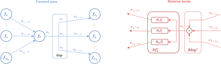
图 8.8：计算图中的反向模式自动微分。Figure 8.8: Reverse mode automatic differentiation in a computation graph.

算法 5 计算图的反向模式自动微分Algorithm 5 Reverse-mode autodiff for computation graphs

1: Functions:

f_{1},\dots,f_{K}

in topological order

2: Inputs: input

{\bm{s}}_{0}\in\mathcal{S}_{0}

, output direction

{\bm{u}}\in\mathcal{S}_{K}

3: for

k\coloneqq 1,\ldots,K

do

\triangleright

Forward pass

4: Retrieve parent nodes

(i_{1},\dots,i_{p_{k}})\coloneqq{\operatorname{pa}}(k)

5: Compute

{\bm{s}}_{k}\coloneqq f_{k}({\bm{s}}_{i_{1}},\ldots,{\bm{s}}_{i_{p_{k}}})\in\mathcal{S}_{k}

6: Instantiate VJP

l_{k}\coloneqq\partial f_{k}({\bm{s}}_{i_{1}},\ldots,{\bm{s}}_{i_{p_{k}}})^{*}

7: Initialize

{\bm{r}}_{K}\coloneqq{\bm{u}}

,

{\bm{r}}_{k}\leftarrow 0 \ \forall k\in\{0,\ldots,K-1\}

\triangleright

Backward pass

8: for

k\coloneqq K,\ldots,1

do

9: Retrieve parent nodes

(i_{1},\dots,i_{p_{k}})\coloneqq{\operatorname{pa}}(k)

10: Compute

{\bm{r}}_{i_{1}\rightarrow k},\dots,{\bm{r}}_{i_{p_{k}}\rightarrow k}\coloneqq l_{k}[{\bm{r}}_{k}]

11: Compute

{\bm{r}}_{i_{j}}\leftarrow{\bm{r}}_{i_{j}}+{\bm{r}}_{i_{j}\rightarrow k}\in\mathcal{S}_{i_{j}} \ \forall j\in\{1,\dots,p_{k}\}

12: Outputs:

f({\bm{s}}_{0})\coloneqq{\bm{s}}_{K}\in\mathcal{S}_{K}

,

\partial f({\bm{s}}_{0})^{*}[{\bm{u}}]={\bm{r}}_{0}\in\mathcal{S}_{0}

例 8.3.1（前向模式与反向模式的示例）Example 8.3.1 (Example of forward and reverse modes).

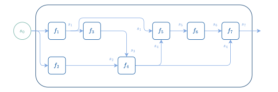
我们用图 8.9 来说明计算图中的前向模式与反向模式。假设中间变量

{\bm{s}}_{1},\dots,{\bm{s}}_{7}

已经计算好。前向模式对应于We use Fig. 8.9 to illustrate the forward and reverse modes in a computation graph. Let us assume that the intermediate variables

{\bm{s}}_{1},\dots,{\bm{s}}_{7}

have readily been computed. The forward mode corresponds to

\displaystyle{\bm{t}}_{0}

\displaystyle\coloneqq{\bm{v}}

\displaystyle{\bm{t}}_{1}

\displaystyle\coloneqq\partial f_{1}({\bm{s}}_{0})[{\bm{t}}_{0}]

\displaystyle{\bm{t}}_{2}

\displaystyle\coloneqq\partial f_{2}({\bm{s}}_{0})[{\bm{t}}_{0}]

\displaystyle{\bm{t}}_{3}

\displaystyle\coloneqq\partial f_{3}({\bm{s}}_{1})[{\bm{t}}_{1}]

\displaystyle{\bm{t}}_{4}

\displaystyle\coloneqq\partial f_{4}({\bm{s}}_{2},{\bm{s}}_{3})[{\bm{t}}_{2},{\bm{t}}_{3}]=\partial_{1}f_{4}({\bm{s}}_{2},{\bm{s}}_{3})[{\bm{t}}_{2}]+\partial_{2}f_{4}({\bm{s}}_{2},{\bm{s}}_{3})[{\bm{t}}_{3}]

\displaystyle{\bm{t}}_{5}

\displaystyle\coloneqq\partial f_{5}({\bm{s}}_{1},{\bm{s}}_{4})[{\bm{t}}_{1},{\bm{t}}_{4}]=\partial_{1}f_{5}({\bm{s}}_{1},{\bm{s}}_{4})[{\bm{t}}_{1}]+\partial_{2}f_{5}({\bm{s}}_{1},{\bm{s}}_{4})[{\bm{t}}_{4}]

\displaystyle{\bm{t}}_{6}

\displaystyle\coloneqq\partial f_{6}({\bm{s}}_{5})[{\bm{t}}_{5}]

\displaystyle{\bm{t}}_{7}

\displaystyle\coloneqq\partial f_{7}({\bm{s}}_{4},{\bm{s}}_{6})[{\bm{t}}_{4},{\bm{t}}_{6}]=\partial_{1}f_{7}({\bm{s}}_{4},{\bm{s}}_{6})[{\bm{t}}_{4}]+\partial_{2}f_{7}({\bm{s}}_{4},{\bm{s}}_{6})[{\bm{t}}_{6}].

反向模式对应于The reverse mode corresponds to

\displaystyle({\bm{r}}_{4\to 7},{\bm{r}}_{6\to 7})

\displaystyle\coloneqq\partial f_{7}({\bm{s}}_{4},{\bm{s}}_{6})^{*}[{\bm{r}}_{7}]\quad

\displaystyle{\bm{r}}_{7}\coloneqq{\bm{u}}

\displaystyle{\bm{r}}_{5\to 6}

\displaystyle\coloneqq\partial f_{6}({\bm{s}}_{5})^{*}[{\bm{r}}_{6}]\quad

\displaystyle{\bm{r}}_{6}\coloneqq{\bm{r}}_{6\to 7}

\displaystyle({\bm{r}}_{1\to 5},{\bm{r}}_{4\to 5})

\displaystyle\coloneqq\partial f_{5}({\bm{s}}_{1},{\bm{s}}_{4})^{*}[{\bm{r}}_{5}]\quad

\displaystyle{\bm{r}}_{5}\coloneqq{\bm{r}}_{5\to 6}

\displaystyle({\bm{r}}_{2\to 4},{\bm{r}}_{3\to 4})

\displaystyle\coloneqq\partial f_{4}({\bm{s}}_{2},{\bm{s}}_{3})^{*}[{\bm{r}}_{4}]\quad

\displaystyle{\bm{r}}_{4}\coloneqq{\bm{r}}_{4\to 5}+{\bm{r}}_{4\to 7}

\displaystyle{\bm{r}}_{1\to 3}

\displaystyle\coloneqq\partial f_{3}({\bm{s}}_{1})^{*}[{\bm{r}}_{3}]\quad

\displaystyle{\bm{r}}_{3}\coloneqq{\bm{r}}_{3\to 4}

\displaystyle{\bm{r}}_{0\to 2}

\displaystyle\coloneqq\partial f_{2}({\bm{s}}_{0})^{*}[{\bm{r}}_{2}]\quad

\displaystyle{\bm{r}}_{2}\coloneqq{\bm{r}}_{2\to 4}

\displaystyle{\bm{r}}_{0\to 1}

\displaystyle\coloneqq\partial f_{1}({\bm{s}}_{0})^{*}[{\bm{r}}_{1}]\quad

\displaystyle{\bm{r}}_{1}\coloneqq{\bm{r}}_{1\to 3}+{\bm{r}}_{1\to 5}

\displaystyle{\bm{r}}_{0}\coloneqq{\bm{r}}_{0\to 1}+{\bm{r}}_{0\to 2}.

图 8.9：与图 4.3 相同的计算图，但为简明起见，省略了每个

f_{k}

的实际定义。Figure 8.9: Same computation graph as Fig. 4.3 but without the actual definition of each

f_{k}

, for simplicity.

8.3.3 复杂度与 Baur-Strassen 定理Complexity, the Baur-Strassen theorem

在计算由计算图表示的函数 $f\colon\mathcal{E}\to\mathbb{R}$ 的梯度时，我们已经看到，反向模式比前向模式更为高效。如前所述，假设 DAG 中各基本函数 $f_{k}$ 及其 VJP 的计算复杂度大致相当，那么 $f$ 与 $\nabla f$ 的计算复杂度也大致相当。这一事实至关重要，现代机器学习正是倚仗它才得以成立：它使我们能够通过梯度下降优化高维函数。For computing the gradient of a function $f\colon\mathcal{E}\to\mathbb{R}$ represented by a computation graph, we saw that the reverse mode is more efficient than the forward mode. As we previously stated, assuming that the elementary functions $f_{k}$ in the DAG and their VJP have roughly the same computational complexity, then $f$ and $\nabla f$ have roughly the same computational complexity. This fact is crucial and is the pillar on which modern machine learning relies: it allows us to optimize high-dimensional functions by gradient descent.

对于 4.1.4 节回顾过的算术电路，这一关键事实在著名的 Baur-Strassen 定理 [14] 中得到了更精确的表述。若 $f$ 是多项式，则其梯度 $\nabla f$ 也是多项式。该定理以计算 $f$ 的最佳电路规模为参照，给出了计算 $\nabla f$ 的最佳电路规模的上界。For arithmetic circuits, reviewed in Section 4.1.4, this crucial fact is made more precise in the celebrated Baur-Strassen theorem [14]. If $f$ is a polynomial, then so is its gradient $\nabla f$ . The theorem gives an upper bound on the size of the best circuit for computing $\nabla f$ from the size of the best circuit for computing $f$ .

命题 8.3.2（Baur-Strassen 定理）Proposition 8.3.2 (Baur-Strassen’s theorem).

对任意多项式

f\colon\mathcal{E}\to\mathbb{R}

，我们有For any polynomial

f\colon\mathcal{E}\to\mathbb{R}

, we have

S(\nabla f)\leq 5\cdot S(f),

其中多项式

f

的规模

S(f)

由定义 4.1.1 给出。where the size

S(f)

of a polynomial

f

is defined in Definition 4.1.1.

[138] 给出了一个借助反向归纳法的更简证明。另见 [44] 中定理 9.10 的证明。对于基本函数不止 $+$ 与 $\times$ 的通用计算图，也可得到类似结果；例如参见 [29，定理 2]。A simpler proof by backward induction was given by [138]. See also the proof of Theorem 9.10 in [44]. For general computation graphs, that have more primitive functions than just $+$ and $\times$ , a similar result can be obtained; see, e.g., [29, Theorem 2].

8.4 实现8.4 Implementation

8.4.1 基本函数Primitive functions

自动微分系统会实现一组基本函数或初等函数 $\mathcal{A}$ ，它们经由函数复合，充当构造其他函数的构件。例如，我们已经看到，在算术电路（4.1.4 节）中有 $\mathcal{A}=\{+,\times\}$ 。更一般地， $\mathcal{A}$ 可以囊括表达程序所需的全部函数。不过我们强调， $\mathcal{A}$ 未必局限于 log、exp 之类的底层函数，也可以包含层次更高的函数。例如，log-sum-exp 虽然可写成基本操作（log、sum、exp）的复合，却通常被单独列为基本函数：这既因为它是极为常用的构件，也因为数值稳定性的考虑。An autodiff system implements a set $\mathcal{A}$ of primitive or elementary functions, which serve as building blocks for creating other functions, by function composition. For instance, we saw that in arithmetic circuits (Section 4.1.4), $\mathcal{A}=\{+,\times\}$ . More generally, $\mathcal{A}$ may contain all the necessary functions for expressing programs. We emphasize, however, that $\mathcal{A}$ is not necessarily restricted to low-level functions such as log and exp, but may also contain higher-level functions. For instance, even though the log-sum-exp can be expressed as the composition of elementary operations (log, sum, exp), it is usually included as a primitive on its own, both because it is a very commonly-used building block, but also for numerical stability reasons.

8.4.2 函数复合下的封闭性Closure under function composition

计算图中的每个函数 $f_{k}$ 都属于一个集合 $\mathcal{F}$ ，即该系统所支持的函数类。自动微分实现的一个理想性质是，集合 $\mathcal{F}$ 在函数复合下封闭，这意味着若 $f\in\mathcal{F}$ 且 $g\in\mathcal{F}$ ，则 $f\circ g\in\mathcal{F}$ 。这意味着复合函数本身可用于构造新的复合函数。这一性质对于支持高阶微分（第 9 章）和自动线性转置（8.4.4 节）也至关重要。当 $f_{k}$ 是 $\mathcal{A}$ 中基本函数的复合时， $f_{k}$ 本身就是一个嵌套的 DAG。不过，我们总可以将每个复合函数内联，使 DAG 中的所有函数都属于 $\mathcal{A}$ 。Each function $f_{k}$ in a computation graph belongs to a set $\mathcal{F}$ , the class of functions supported by the system. A desirable property of an autodiff implementation is that the set $\mathcal{F}$ is closed under function composition, meaning that if $f\in\mathcal{F}$ and $g\in\mathcal{F}$ , then $f\circ g\in\mathcal{F}$ . This means that composed functions can themselves be used for composing new functions. This property is also crucial for supporting higher-order differentiation (Chapter 9) and automatic linear transposition (Section 8.4.4). When $f_{k}$ is a composition of elementary functions in $\mathcal{A}$ , then $f_{k}$ itself is a nested DAG. However, we can always inline each composite function, such that all functions in the DAG belong to $\mathcal{A}$ .

8.4.3 JVP 与 VJP 的示例Examples of JVPs and VJPs

自动微分系统必须为每个 $f\in\mathcal{A}$ 实现其 JVP 以支持前向模式，并实现其 VJP 以支持反向模式。我们给出几个示例，首先从线性函数的 JVP 与 VJP 开始。An autodiff system must implement for each $f\in\mathcal{A}$ its JVP for supporting the forward mode, and its VJP for supporting the reverse mode. We give a couple of examples. We start with the JVP and VJP of linear functions.

例 8.4.1（线性函数的 JVP 与 VJP）。Example 8.4.1 (JVP and VJP of linear functions).

考虑矩阵—向量乘法

f({\bm{W}})={\bm{W}}{\bm{x}}\in\mathbb{R}^{M}

，其中

{\bm{x}}\in\mathbb{R}^{D}

固定，且

{\bm{W}}\in\mathbb{R}^{M\times D}

。正如第 2.3.1 节已经提到的，

f

在

{\bm{W}}\in\mathbb{R}^{M\times D}

处沿输入方向

{\bm{V}}\in\mathbb{R}^{M\times D}

的 JVP 就是Consider the matrix-vector product

f({\bm{W}})={\bm{W}}{\bm{x}}\in\mathbb{R}^{M}

, where

{\bm{x}}\in\mathbb{R}^{D}

is fixed and

{\bm{W}}\in\mathbb{R}^{M\times D}

. As already mentioned in Section 2.3.1, the JVP of

f

at

{\bm{W}}\in\mathbb{R}^{M\times D}

along an input direction

{\bm{V}}\in\mathbb{R}^{M\times D}

is simply

\partial f({\bm{W}})[{\bm{V}}]=f({\bm{V}})={\bm{V}}{\bm{x}}\in\mathbb{R}^{M}.

为求出相应的 VJP，我们注意到：对任意

{\bm{u}}\in\mathbb{R}^{M}

和

{\bm{V}}\in\mathbb{R}^{M\times D}

，都必须有

\langle\partial f({\bm{W}})[{\bm{V}}],{\bm{u}}\rangle=\langle{\bm{V}},\partial f({\bm{W}})^{*}[{\bm{u}}]\rangle

。利用迹的性质，可得To find the associated VJP, we note that for any

{\bm{u}}\in\mathbb{R}^{M}

and

{\bm{V}}\in\mathbb{R}^{M\times D}

, we must have

\langle\partial f({\bm{W}})[{\bm{V}}],{\bm{u}}\rangle=\langle{\bm{V}},\partial f({\bm{W}})^{*}[{\bm{u}}]\rangle

. Using the properties of the trace, we have

\langle\partial f({\bm{W}})[{\bm{V}}],{\bm{u}}\rangle=\langle{\bm{V}}{\bm{x}},{\bm{u}}\rangle=\operatorname{tr}({\bm{x}}^{\top}{\bm{V}}^{\top}{\bm{u}})=\langle{\bm{V}},{\bm{u}}{\bm{x}}^{\top}\rangle.

因此，VJP 由下式给出Therefore, we find that the VJP is given by

\partial f({\bm{W}})^{*}[{\bm{u}}]={\bm{u}}{\bm{x}}^{\top}\in\mathbb{R}^{M\times D}.

类似地，现在考虑矩阵—矩阵乘积

f({\bm{W}})={\bm{W}}{\bm{X}}

，其中

{\bm{W}}\in\mathbb{R}^{M\times D}

，且

{\bm{X}}\in\mathbb{R}^{D\times N}

固定。在

{\bm{W}}\in\mathbb{R}^{M\times D}

处沿输入方向

{\bm{V}}\in\mathbb{R}^{M\times D}

的 JVP 就是Similarly, consider now a matrix-matrix product

f({\bm{W}})={\bm{W}}{\bm{X}}

, where

{\bm{W}}\in\mathbb{R}^{M\times D}

and where

{\bm{X}}\in\mathbb{R}^{D\times N}

is fixed. The JVP at

{\bm{W}}\in\mathbb{R}^{M\times D}

along an input direction

{\bm{V}}\in\mathbb{R}^{M\times D}

is simply

\partial f({\bm{W}})[{\bm{V}}]=f({\bm{V}})={\bm{V}}{\bm{X}}\in\mathbb{R}^{M\times N}.

沿输出方向

{\bm{U}}\in\mathbb{R}^{M\times N}

的 VJP 为The VJP along the output direction

{\bm{U}}\in\mathbb{R}^{M\times N}

is

\partial f({\bm{W}})^{*}[{\bm{U}}]={\bm{U}}{\bm{X}}^{\top}\in\mathbb{R}^{M\times D}.

另一个简单的例子是逐元素可分离函数。Another simple example is element-wise separable functions.

例 8.4.2（可分离函数的 JVP 与 VJP）。Example 8.4.2 (JVP and VJP of separable function).

考虑函数

f({\bm{w}})\coloneqq(g_{1}(w_{1}),\dots,g_{P}(w_{P}))

，其中每个

g_{i}\colon\mathbb{R}\to\mathbb{R}

的导数为

g_{i}^{\prime}

。此时雅可比矩阵是一个对角矩阵Consider the function

f({\bm{w}})\coloneqq(g_{1}(w_{1}),\dots,g_{P}(w_{P}))

, where each

g_{i}\colon\mathbb{R}\to\mathbb{R}

has a derivative

g_{i}^{\prime}

. The Jacobian matrix is then a diagonal matrix

\bm{\partial}f({\bm{w}})=\operatorname{\bf diag}(g_{1}^{\prime}(w_{1}),\dots,g_{P}^{\prime}(w_{P}))\in\mathbb{R}^{P\times P}.

在这种情况下，JVP 与 VJP 实际上相同In this case, the JVP and VJP are actually the same

\partial f({\bm{w}})[{\bm{v}}]=\partial f({\bm{w}})^{*}[{\bm{v}}]=(g_{1}^{\prime}(w_{1}),\dots,g_{P}^{\prime}(w_{P}))\odot{\bm{v}},

其中

\odot

表示逐元素乘积。where

\odot

indicates element-wise multiplication.

8.4.4 自动线性转置Automatic linear transposition

乍看之下，若要同时支持前向模式与反向模式，似乎需要为每个基本操作 $f\in\mathcal{A}$ 同时实现 JVP 与 VJP。幸运的是，存在一种从 JVP 得到 VJP 的方法，反之亦然。On first sight, if we want to support both forward and reverse modes, it appears like we need to implement both the JVP and the VJP for each primitive operation $f\in\mathcal{A}$ . Fortunately, there exists a way to recover VJPs from JVPs, and vice-versa.

如 2.3 节所示，若 $l({\bm{w}})$ 是线性映射，则其 JVP 为 $\partial l({\bm{w}})[{\bm{v}}]=l({\bm{v}})$ （与 ${\bm{w}}$ 无关）。反之，其 VJP 为 $\partial l({\bm{w}})^{*}[{\bm{u}}]=l^{*}({\bm{u}})$ ，其中 $l^{*}$ 是 $l$ 的伴随算子（同样与 ${\bm{w}}$ 无关）。We saw in Section 2.3 that if $l({\bm{w}})$ is a linear map, then its JVP is $\partial l({\bm{w}})[{\bm{v}}]=l({\bm{v}})$ (independent of ${\bm{w}}$ ). Conversely, the VJP is $\partial l({\bm{w}})^{*}[{\bm{u}}]=l^{*}({\bm{u}})$ , where $l^{*}$ is the adjoint operator of $l$ (again, independent of ${\bm{w}}$ ).

我们定义 $l({\bm{u}};{\bm{w}})\coloneqq\partial f({\bm{w}})^{*}[{\bm{u}}]$ ，即 $f$ 在输出方向 ${\bm{u}}$ 上的 VJP。由于 $l({\bm{u}};{\bm{w}})$ 关于 ${\bm{u}}$ 是线性的，我们可以运用上述推理来计算其 VJPLet us define $l({\bm{u}};{\bm{w}})\coloneqq\partial f({\bm{w}})^{*}[{\bm{u}}]$ , i.e., the VJP of $f$ in the output direction ${\bm{u}}$ . Since $l({\bm{u}};{\bm{w}})$ is linear in ${\bm{u}}$ , we can apply the reasoning above to compute its VJP

\partial l({\bm{u}};{\bm{w}})^{*}[{\bm{v}}]=l^{*}({\bm{v}};{\bm{w}})=\partial f({\bm{w}})^{**}[{\bm{v}}]=\partial f({\bm{w}})[{\bm{v}}],

它与 ${\bm{u}}$ 无关。换言之，VJP 的 VJP 正是对应的 JVP！这意味着，即使我们只能访问 VJP，也能实现前向模式自动微分。作为说明与合理性检验，我们给出下面的例子。which is independent of ${\bm{u}}$ . In words, the VJP of a VJP is the corresponding JVP! This means that we can implement forward-mode autodiff even if we only have access to VJPs. As an illustration and sanity check, we give the following example.

例 8.4.3（“点积”的自动转置）。Example 8.4.3 (Automatic transpose of “dot”).

若定义

f({\bm{x}},{\bm{W}})\coloneqq{\bm{W}}{\bm{x}}

，则由例 8.4.1 可知If we define

f({\bm{x}},{\bm{W}})\coloneqq{\bm{W}}{\bm{x}}

, from Example 8.4.1, we know that

\displaystyle\partial f({\bm{x}},{\bm{W}})^{*}[{\bm{u}}]

\displaystyle=({\bm{W}}^{\top}{\bm{u}},{\bm{u}}{\bm{x}}^{\top})

\displaystyle=(f({\bm{u}},{\bm{W}}^{\top}),f({\bm{x}}^{\top},{\bm{u}}))

\displaystyle\eqqcolon l({\bm{u}};{\bm{x}},{\bm{W}}).

利用命题 2.3.16，我们得到Using Proposition 2.3.16, we obtain

\displaystyle\partial l({\bm{u}};{\bm{x}},{\bm{W}})^{*}[{\bm{v}},{\bm{V}}]

\displaystyle=f({\bm{v}},{\bm{W}})+f({\bm{x}},{\bm{V}})

\displaystyle={\bm{W}}{\bm{v}}+{\bm{V}}{\bm{x}}

\displaystyle=\partial f({\bm{x}},{\bm{W}})[{\bm{v}},{\bm{V}}].

另一个方向，即从 JVP 自动构造 VJP，同样可行，但技术性更强，并依赖于部分求值（partial evaluation）这一概念 [73, 164]。The other direction, automatically creating a VJP from a JVP, is also possible but is more technical and relies on the notion of partial evaluation [73, 164].

8.5 检查点8.5 Checkpointing

我们已经看到，前向模式自动微分可以在计算过程中释放中间计算所占用的内存，而反向模式自动微分则需要缓存所有这些中间计算。这意味着，在标准形式下，反向模式自动微分的内存复杂度会随计算图中节点数量线性增长。规避这一问题的一种常用技术是检查点，它通过牺牲计算时间来换取更好的内存使用。检查点的工作方式是：只选择性地存储中间值的一个子集（称为检查点），并在需要时重新计算其余中间值。计算图中检查点位置的具体选择决定了内存与计算之间的权衡。虽然可以按用户指定的位置凭经验设置检查点，但检查点策略也可以按照算法来执行，[84, 87] 对此进行了深入研究。本节回顾两种分治算法：递归折半与动态规划。我们的阐述聚焦于计算链 $f=f_{K}\circ\ldots\circ f_{1}$ ，为简单起见取 $f_{k}:\mathbb{R}^{D}\rightarrow\mathbb{R}^{D}$ 。We saw that forward-mode autodiff can release intermediate computations from memory along the way, while reverse-mode autodiff needs to cache all of them. This means that the memory complexity of reverse-mode autodiff, in its standard form, grows linearly with the number of nodes in the computation graph. A commonly-used technique to circumvent this issue is checkpointing, which trades-off computation time for better memory usage. Checkpointing works by selectively storing only a subset of the intermediate values, called checkpoints, and by recomputing others on the fly. The specific choice of the checkpoint locations in the computation graph determines the memory-computation trade-off. While it is possible to heuristically set checkpoints at user-specified locations, it is also possible to perform a checkpointing strategy algorithmically, as studied in depth by [84, 87]. In this section, we review two divide-and-conquer algorithms: recursive halving and dynamic programming. Our exposition focuses on computation chains $f=f_{K}\circ\ldots\circ f_{1}$ , with $f_{k}:\mathbb{R}^{D}\rightarrow\mathbb{R}^{D}$ for simplicity.

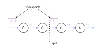
图 8.10：检查点通过选择性地只存储中间值的一个子集（称为检查点），并在需要时重新计算其余中间值，以计算时间换取更好的内存使用。递归折半与动态规划是两种用于选择检查点位置的分治策略。Figure 8.10: Checkpointing trades-off computation time for better memory usage by selectively storing only a subset of the intermediate values, called checkpoints, and by recomputing others on the fly. Recursive halving and dynamic programming are two divide-and-conquer strategies to select the checkpoint locations.

两个极端情形下的计算复杂度与内存复杂度Computational and memory complexities at two extremes

设 $\mathcal{C}(K)$ 为对各个函数 $f_{k}$ 的调用次数（我们忽略计算中间 VJP 的代价）， $\mathcal{M}(K)$ 为对链 $f=f_{K}\circ\ldots\circ f_{1}$ 执行反向模式自动微分时缓存的函数输入个数。在一个极端，如果像算法 2 那样存储所有中间计算，以仅计算 VJP $\partial f({\bm{s}}_{0})^{*}[{\bm{u}}]$ ，则我们有Let $\mathcal{C}(K)$ be the number of calls to the individual functions $f_{k}$ (we ignore the cost of computing the intermediate VJPs) and $\mathcal{M}(K)$ be the number of function inputs cached, when performing reverse-mode autodiff on a chain $f=f_{K}\circ\ldots\circ f_{1}$ . On one extreme, if we store all intermediate computations, as done in Algorithm 2, to compute only the VJP $\partial f({\bm{s}}_{0})^{*}[{\bm{u}}]$ , we have

\mathcal{C}(K)=K-1\quad\text{and}\quad\mathcal{M}(K)=K.

这在计算复杂度上是最优的，但在内存上则不是最优的。在另一个极端，如果像算法 6 那样只存储初始输入，则我们有This is optimal w.r.t. computational complexity, but suboptimal w.r.t. memory. On the other extreme, if we only store the initial input, as done in Algorithm 6, then we have

\mathcal{C}(K)=K(K-1)/2\quad\text{and}\quad\mathcal{M}(K)=1.

这在内存上是最优的，但会导致计算复杂度关于 $K$ 呈二次增长。This is optimal w.r.t. memory but leads to a computational complexity that is quadratic in $K$ .

算法 6 常数内存下的反向模式自动微分

\texttt{vjp\_full\_recompute}(f_{K}\circ\ldots\circ f_{1},{\bm{s}}_{0},{\bm{u}})\coloneqq\partial(f_{K}\circ\ldots\circ f_{1})({\bm{s}}_{0})^{*}[{\bm{u}}]

Algorithm 6 Reverse-mode autodiff with constant memory

\texttt{vjp\_full\_recompute}(f_{K}\circ\ldots\circ f_{1},{\bm{s}}_{0},{\bm{u}})\coloneqq\partial(f_{K}\circ\ldots\circ f_{1})({\bm{s}}_{0})^{*}[{\bm{u}}]

1: Inputs: Chain

f_{K}\circ\ldots\circ f_{1}

, input

{\bm{s}}_{0}\in\mathcal{S}_{0}

, output direction

{\bm{u}}\in\mathcal{S}_{K}

2: if

K=1

then

3: return

\partial f_{1}({\bm{s}}_{0})^{*}[{\bm{u}}]

4: else

5: Set

{\bm{r}}_{K}={\bm{u}}

6: for

k\coloneqq K,\ldots,1

do

7: Compute

{\bm{s}}_{k-1}=(f_{k-1}\circ\ldots\circ f_{1})({\bm{s}}_{0})

8: Compute

{\bm{r}}_{k-1}=\partial f_{k}({\bm{s}}_{k-1})^{*}[{\bm{r}}_{k}]

9: return:

{\bm{r}}_{0}

8.5.1 递归折半Recursive halving

作为在计算与内存之间获得更好权衡的第一步，我们可以将链 ${\bm{s}}_{K}=f_{K}\circ\dots\circ f_{1}({\bm{s}}_{0})$ 拆分为As a first step towards obtaining a better computation-memory trade-off, we may split the chain ${\bm{s}}_{K}=f_{K}\circ\dots\circ f_{1}({\bm{s}}_{0})$ as

$\displaystyle{\bm{s}}_{K/2}$	$\displaystyle=f_{K/2}\circ\ldots\circ f_{1}({\bm{s}}_{0})$
$\displaystyle{\bm{s}}_{K}$	$\displaystyle=f_{K}\circ\ldots\circ f_{K/2+1}({\bm{s}}_{K/2}),$

其中 $K$ 为偶数。于是，不同于像算法 6 那样从输入 ${\bm{s}}_{0}$ 重新计算所有中间计算 ${\bm{s}}_{k}$ ，我们可以存储 ${\bm{s}}_{K/2}$ ，并从 ${\bm{s}}_{K/2}$ 出发对 $k>K/2$ 重新计算 ${\bm{s}}_{k}$ 。形式化地说，该策略对应于以下步骤。for $K$ even. Then, rather than recomputing all intermediate computations ${\bm{s}}_{k}$ from the input ${\bm{s}}_{0}$ as in Algorithm 6, we can store ${\bm{s}}_{K/2}$ and recompute ${\bm{s}}_{k}$ for $k>K/2$ starting from ${\bm{s}}_{K/2}$ . Formally, this strategy amounts to the following steps.

1.

计算 ${\bm{s}}_{K/2}=f_{K/2}\circ\ldots\circ f_{1}({\bm{s}}_{0})$ Compute ${\bm{s}}_{K/2}=f_{K/2}\circ\ldots\circ f_{1}({\bm{s}}_{0})$
2.

计算 ${\bm{r}}_{K/2}=\text{{vjp\_full\_recompute}}(f_{K}\circ\ldots\circ f_{K/2+1},{\bm{s}}_{K/2},{\bm{u}})$ Compute ${\bm{r}}_{K/2}=\text{{vjp\_full\_recompute}}(f_{K}\circ\ldots\circ f_{K/2+1},{\bm{s}}_{K/2},{\bm{u}})$
3.

计算 ${\bm{r}}_{0}=\text{{vjp\_full\_recompute}}(f_{K/2}\circ\ldots\circ f_{1},{\bm{s}}_{0},{\bm{r}}_{K/2})$ Compute ${\bm{r}}_{0}=\text{{vjp\_full\_recompute}}(f_{K/2}\circ\ldots\circ f_{1},{\bm{s}}_{0},{\bm{r}}_{K/2})$

代价是需要额外存储检查点 ${\bm{s}}_{K/2}$ ；但与算法 6 相比，这已把计算复杂度大致减半。At the expense of having to store the additional checkpoint ${\bm{s}}_{K/2}$ , this already roughly halves the computational complexity compared to Algorithm 6.

算法 7 带递归折半的反向模式自动微分

\texttt{vjp\_halving}(f_{K}\circ\ldots\circ f_{1},{\bm{s}}_{0},{\bm{u}})\coloneqq\partial(f_{K}\circ\ldots\circ f_{1})({\bm{s}}_{0})^{*}[{\bm{u}}]

Algorithm 7 Reverse-mode autodiff with recursive halving

\texttt{vjp\_halving}(f_{K}\circ\ldots\circ f_{1},{\bm{s}}_{0},{\bm{u}})\coloneqq\partial(f_{K}\circ\ldots\circ f_{1})({\bm{s}}_{0})^{*}[{\bm{u}}]

1: Functions: Chain

f_{K}\circ\ldots\circ f_{1}

2: Inputs: input

{\bm{s}}_{0}\in\mathcal{S}_{0}

, output direction

{\bm{u}}\in\mathcal{S}_{K}

3: if

K=1

then

4: return

\partial f_{1}({\bm{s}}_{0})^{*}[{\bm{u}}]

5: else

6: Compute

{\bm{s}}_{K/2}=f_{K/2}\circ\ldots\circ f_{1}({\bm{s}}_{0})

7: Compute

{\bm{r}}_{K/2}=\text{{vjp\_halving}}(f_{K}\circ\ldots\circ f_{K/2+1},{\bm{s}}_{K/2},{\bm{u}})

8: Compute

{\bm{r}}_{0}=\text{{vjp\_halving}}(f_{K/2}\circ\ldots\circ f_{1},{\bm{s}}_{0},{\bm{r}}_{K/2})

9: return:

{\bm{r}}_{0}

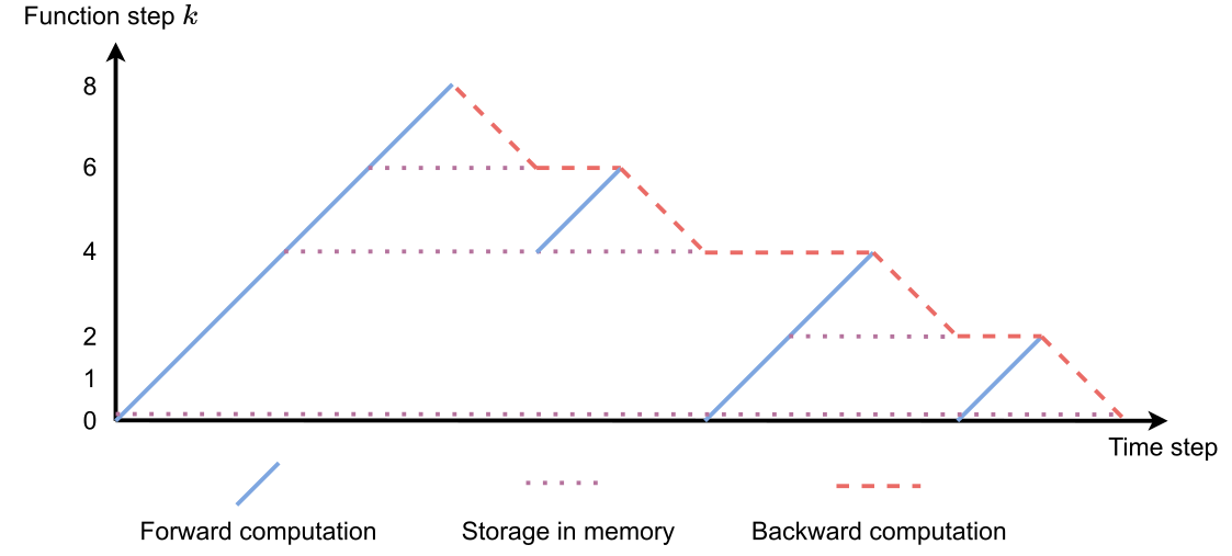
随后便可递归地应用这一推理，算法 7 即其形式化表述。该算法称为递归二分调度 [85]，图 8.11 给出了图示。就函数求值次数 $\mathcal{C}(K)$ 而言，当 $K$ 为偶数时，我们进行 $K/2$ 次函数调用，并将该过程递归调用两次，即，We can then apply this reasoning recursively, as formalized in Algorithm 7. The algorithm is known as recursive binary schedule [85] and illustrated in Fig. 8.11. In terms of number of function evaluations $\mathcal{C}(K)$ , for $K$ even, we make $K/2$ function calls, and we call the procedure recursively twice, that is,

\displaystyle\mathcal{C}(K)

\displaystyle=2\mathcal{C}(K/2)+K/2.

若链的长度为 $1$ ，我们直接使用 VJP，因此 $\mathcal{C}(1)=0$ 。于是，若 $K$ 是 $2$ 的幂，函数调用次数为If the chain is of length $1$ , we directly use the VJP, so $\mathcal{C}(1)=0$ . Hence, the number of function calls, if $K$ is a power of $2$ , is

\mathcal{C}(K)=\frac{K}{2}\log_{2}K.

就内存占用而言，算法 7 不仅在第 6 行使用 ${\bm{s}}_{0}$ ，在第 8 行也同样使用。因此，当算法在第 7 行对链的后半部分进行递归调用时，一个内存槽被 ${\bm{s}}_{0}$ 占用。该行被递归调用，直至链缩减为单个函数。此时，所使用的内存槽总数等于我们将函数折半的次数，即当 $K$ 是 $2$ 的幂时为 $\log_{2}K$ 。另一方面，输入 ${\bm{s}}_{0}$ 在算法 7 的第 8 行之后不再被使用。在该行， ${\bm{s}}_{0}$ 所占用的内存槽可由对前半部分的递归调用使用。换言之，对前半部分递归调用算法不会带来额外的内存开销。因此，若 $K$ 是 $2$ 的幂，算法 7 的内存开销为In terms of memory usage, Algorithm 7 uses ${\bm{s}}_{0}$ not only at line 6 but also at line 8. So when the algorithm is called recursively on the second half of the chain at line 7, one memory slot is taken by ${\bm{s}}_{0}$ . This line is called recursively until the chain is reduced to a single function. At that point, the total number of memory slots used is equal to the number of times we split the function in half, that is, $\log_{2}K$ for $K$ a power of $2$ . On the other hand, the input ${\bm{s}}_{0}$ is no longer used after line 8 of Algorithm 7. At that line, the memory slot taken by ${\bm{s}}_{0}$ can be consumed by the recursive call on the first-half. In other words, calling the algorithm recursively on the first half does not incur extra memory cost. So if $K$ is a power of $2$ , the memory cost of Algorithm 7 is

\mathcal{M}(K)=\log_{2}K.

图 8.11：对由

8

个函数组成的链使用递归折半进行检查点技术的图示。首先对链进行完整求值，同时将一些计算作为检查点存入内存。随后，在反向传播过程中，我们从可用的最新检查点重新计算部分中间值。相比之下，朴素的反向模式自动微分（完整缓存中间计算）会呈现一个简单的三角形。Figure 8.11: Illustration of checkpointing with recursive halving, for a chain of

8

functions. The chain is first fully evaluated while storing some computations as checkpoints in memory. Then, during the backward pass, we recompute some intermediate values from the latest checkpoint available. In contrast, vanilla reverse-mode autodiff (with full caching of the intermediate computations) would lead to a simple triangle shape.

8.5.2 动态规划Dynamic programming

对于长度为 $K$ 的链，递归折半需要 $\log_{2}K$ 个内存槽。然而，如图 8.11 所示，在给定时间步，并非所有内存槽都会被利用。Recursive halving requires $\log_{2}K$ memory slots for a chain of length $K$ . However, as illustrated in Fig. 8.11, at a given time step, all memory slots may not be exploited.

为改进这一方法，我们注意到递归折半不过是“将链拆分、再对每一部分递归调用自身”这类程序的一个特例。换言之，它属于分治算法。与其把链对半拆开，不如考虑在某个索引 $l$ 处将其拆分：一部分通过一次递归调用来反转从 $l+1$ 到 $K$ 的计算，该调用会占用一个内存槽；另一部分同样通过递归调用来反转从 $0$ 到 $l$ 的计算，而这次调用无需额外内存槽，因为它可以直接复用原始输入 ${\bm{s}}_{0}$ 所占用的内存槽。要把链拆成这两部分，需要 $l$ 次中间计算，以从 ${\bm{s}}_{0}$ 推进到 ${\bm{s}}_{l}$ 。于是，对于长度为 $k$ 、拥有 $s$ 个内存槽的链，其计算复杂度 $\mathcal{C}(k,s)$ （以函数求值次数计）满足递推式To optimize the approach, we observe that recursive halving is just one instance of a program that splits the chain and calls itself recursively on each part. In other words, it is a form of divide-and-conquer algorithm. Rather than splitting the chain in half, we may consider splitting the chain at some index $l$ . One split is used to reverse the computations from $l+1$ to $K$ by a recursive call that consumes one memory slot. The other split is used on a recursive call that reverses the computations from $0$ to $l$ . That second call does not require an additional memory slot, as it can use directly the memory slot used by the original input ${\bm{s}}_{0}$ . To split the chain in such two parts, we need $l$ intermediate computations to go from ${\bm{s}}_{0}$ to ${\bm{s}}_{l}$ . The computational complexity $\mathcal{C}(k,s)$ , counted as the number of function evaluations, for a chain of length $k$ with $s$ memory slots then satisfies the recurrence

\mathcal{C}(k,s)=\mathcal{C}(k-l,s-1)+\mathcal{C}(l,s)+l,

对一切 $l\in\{1,\dots,k-1\}$ 成立。只需取 $l=k/2$ ，得到的结果恰好就是递归折半的计算复杂度。为进一步优化后者，可以选取合适的 $l$ 来拆分链，使复杂度最小。一个最优方案必须满足如下递推方程：for all $l\in\{1,\dots,k-1\}$ . By simply taking $l=k/2$ , we recover exactly the computational complexity of recursive halving. To refine the latter, we may split the chain by selecting $l$ to minimize the complexity. An optimal scheme must satisfy the recursive equation,

\mathcal{C}^{*}(k,s)\coloneqq\min_{1\leq l\leq k-1}\{\mathcal{C}^{*}(k-l,s-1)+\mathcal{C}^{*}(l,s)+l\}.

(8.3)

注意到对 $k=1,\ldots,K-1$ 、 $s=1,\ldots,S-1$ ， $\mathcal{C}^{*}(K,S)$ 可由 $\mathcal{C}^{*}(k,s)$ 算出。这提示可以采用动态规划方法，通过算法寻找最优方案。对于长度为 $k=1$ 的链，由于可以直接反转计算，代价为零，故 $\mathcal{C}^{*}(1,s)\coloneqq 0$ 。而对于内存 $s=1$ ，只存在一种可行方案，即如算法 6 那样仅保存初始输入，故 $\mathcal{C}^{*}(k,1)\coloneqq(k(k-1))/2$ 。随后可借助式 8.3，从 $k=1$ 到 $K$ 、以及从 $s=1$ 到 $S$ 逐步递推计算各值 $\mathcal{C}^{*}(k,s)$ 。在此过程中，可将最优拆分记录如下：Note that $\mathcal{C}^{*}(K,S)$ can be computed from $\mathcal{C}^{*}(k,s)$ for $k=1,\ldots,K-1$ , $s=1,\ldots,S-1$ . This suggests a dynamic programming approach to find an optimal scheme algorithmically. For a chain of length $k=1$ , the cost is null as we directly reverse the computation, so $\mathcal{C}^{*}(1,s)\coloneqq 0$ . On the other hand for a memory $s=1$ , there is only one possible scheme that saves only the initial input as in Algorithm 6, so $\mathcal{C}^{*}(k,1)\coloneqq(k(k-1))/2$ . The values $\mathcal{C}^{*}(k,s)$ can then be computed incrementally from $k=1$ to $K$ and $s=1$ to $S$ using Eq. 8.3. The optimal splits can be recorded along the way as

l^{*}(k,s)\coloneqq\argmin_{1\leq l\leq k-1}\{\mathcal{C}^{*}(k-l,s-1)+\mathcal{C}^{*}(l,s)+l\}.

随后，通过沿分别对应 $\mathcal{C}^{*}(k-l,s-1)$ 与 $\mathcal{C}^{*}(l,s)$ 的两条分支回溯最优拆分，即可求得 $K,S$ 的最优拆分。由于最终输出表现为遍历一棵二叉树，该方案被称为 treeverse [84]。值得注意的是，这一动态规划流程具有通用性，原则上可以纳入中间函数 $f_{k}$ 的不同计算代价。The optimal split for $K,S$ can then be found by backtracking the optimal splits along both branches corresponding to $\mathcal{C}^{*}(k-l,s-1)$ and $\mathcal{C}^{*}(l,s)$ . As the final output consists in traversing a binary tree, it was called treeverse [84]. Note that the dynamic programming procedure is generic and could a priori incorporate varying computational costs for the intermediate functions $f_{k}$ .

解析公式Analytical formula

结果表明，我们也可以解析地找到一种最优方案。该方案由 [84] 提出，依据的是 [88] 关于分治算法如何最优地反转顺序程序的分析；简明的证明亦可参见 [85，第 6 节]。其主要思路在于考察某个求值步骤 $f_{k}$ 被重复的次数。当我们在 $l$ 处将计算链拆分时，从 $1$ 到 $l$ 的所有步骤都至少会被重复一次。换言之，处理计算链的后半部分会带来一次内存代价，而处理其前半部分则会带来一次重复代价。[84] 表明，对于固定的 $K$ 、 $S$ ，我们可以解析地求出最小重复次数，并借助关于最优拆分的简单公式构造出相应的方案。It turns out that we can also find an optimal scheme analytically. This scheme was found by [84], following the analysis of optimal inversions of sequential programs by divide-and-conquer algorithms done by [88]; see also [85, Section 6] for a simple proof. The main idea consists in considering the number of times an evaluation step $f_{k}$ is repeated. As we split the chain at $l$ , all steps from $1$ to $l$ will be repeated at least once. In other words, treating the second half of the chain incurs one memory cost, while treating the first half of the chain incurs one repetition cost. [84] shows that for fixed $K$ , $S$ , we can find the minimal number of repetitions analytically and build the corresponding scheme with simple formulas for the optimal splits.

与动态规划方法相比，这意味着我们无需计算指针 $l^{*}(k,s)$ ，并且可以用一个简单的公式来设定 $l^{*}(k,s)$ 。在给定 $K,S$ 与 $l^{*}(k,s)$ 的情况下，我们仍需遍历相应的二叉树以获得调度方案。需要注意的是，这种最优方案并未考虑各函数 $f_{k}$ 的计算代价可能不同。Compared to the dynamic programming approach, it means that we do not need to compute the pointers $l^{*}(k,s)$ , and we can use a simple formula to set $l^{*}(k,s)$ . We still need to traverse the corresponding binary tree given $K,S$ and $l^{*}(k,s)$ to obtain the schedules. Note that such an optimal scheme does not take into account varying computational costs for the functions $f_{k}$ .

8.5.3 在线检查点Online checkpointing

上文给出的最优方案要求事先知道计算图中的节点总数。然而，当通过例如 while 循环（5.10 节）进行求导时，情况并非如此。为规避这一问题，研究者提出了在线检查点方案，并证明其近乎最优 [188, 207]。这类方案先以前 $S$ 次计算定义一组共 $S$ 个检查点，随后随着计算的持续进行动态地重写这些检查点。一旦计算终止，就对所记录的检查点集合应用上文针对固定长度给出的最优方法。The optimal scheme presented above requires knowing the total number of nodes in the computation graph ahead of time. However, when differentiating through for example a while loop (Section 5.10), this is not the case. To circumvent this issue, online checkpointing schemes have been developed and proven to be nearly optimal [188, 207]. These schemes start by defining a set of $S$ checkpoints with the first $S$ computations, then these checkpoints are rewritten dynamically as the computations keep going. Once the computations terminate, the optimal approach presented above for a fixed length is applied on the set of checkpoints recorded.

8.6 可逆层8.6 Reversible layers

8.6.1 一般情形General case

当函数 $f_{k}$ 可逆（即 $f_{k}^{-1}$ 存在）且 $f_{k}^{-1}$ 易于获取时，反向模式自动微分的内存需求可以被完全消除。在这种情况下，我们无需存储计算 VJP ${\bm{r}}_{k}\mapsto\partial f_{k}({\bm{s}}_{k-1})^{*}[{\bm{r}}_{k}]$ 所必需的中间计算结果 ${\bm{s}}_{k-1}$ ，而是在反向传播过程中利用 ${\bm{s}}_{k-1}=f_{k}^{-1}({\bm{s}}_{k})$ 从 ${\bm{s}}_{k}$ 即时计算得到。算法 8 针对计算链的情形总结了这一流程。与算法 2 中朴素的反向模式自动微分相比，该算法具有最优的内存复杂度，因为我们可以随计算推进及时释放 ${\bm{s}}_{k}$ 与 ${\bm{r}}_{k}$ 。The memory requirements of reverse-mode autodiff can be completely alleviated when the functions $f_{k}$ are invertible (meaning that $f_{k}^{-1}$ exists) and when $f_{k}^{-1}$ is easily accessible. In that case, rather than storing the intermediate computations ${\bm{s}}_{k-1}$ , necessary to compute the VJP ${\bm{r}}_{k}\mapsto\partial f_{k}({\bm{s}}_{k-1})^{*}[{\bm{r}}_{k}]$ , one can compute them on the fly during the backward pass from ${\bm{s}}_{k}$ using ${\bm{s}}_{k-1}=f_{k}^{-1}({\bm{s}}_{k})$ . We summarize the procedure for the case of computation chains in Algorithm 8. Compared to vanilla reverse-mode autodiff in Algorithm 2, the algorithm has optimal memory complexity, as we can release ${\bm{s}}_{k}$ and ${\bm{r}}_{k}$ as we go.

算法 8 可逆链的反向模式自动微分。Algorithm 8 Reverse-mode autodiff for reversible chains.

1: Functions:

f\coloneqq f_{K}\circ\ldots\circ f_{1}

, with each

f_{k}

invertible

2: Inputs: input

{\bm{s}}_{0}\in\mathcal{S}_{0}

, output direction

{\bm{u}}\in\mathcal{S}_{K}

3: Compute

{\bm{s}}_{K}=f_{K}\circ\ldots\circ f_{1}({\bm{s}}_{0})

4: for

k\coloneqq K,\ldots,1

do

5: Compute

{\bm{s}}_{k-1}=f_{k}^{-1}({\bm{s}}_{k})

6: Compute

{\bm{r}}_{k-1}=\partial f_{k}({\bm{s}}_{k-1})^{*}[{\bm{r}}_{k}]

7: Outputs:

f({\bm{s}}_{0})\coloneqq{\bm{s}}_{K}

,

\partial f({\bm{s}}_{0})^{*}[{\bm{u}}]={\bm{r}}_{0}

实践中， $f_{k}^{-1}$ 往往并不存在，或者不易获取。但是，可以把网络架构设计得易于求逆。这方面的例子包括可逆残差网络 [81]、正交归一 RNN [92]、神经常微分方程（12.6 节）以及动量残差神经网络 [174]；亦可参见其中所引文献。In practice, $f_{k}^{-1}$ often does not exist or may not be easily accessible. However, network architectures can be constructed to be easily invertible by design. Examples include reversible residual networks [81], orthonormal RNNs [92], neural ODEs (Section 12.6), and momentum residual neural networks [174]; see also references therein.

8.6.2 正交归一 JVP 的情形Case of orthonormal JVPs

当每个 $f_{k}$ 的 JVP 都是正交归一的线性映射时，即When the JVP of each $f_{k}$ is an orthonormal linear mapping, i.e.,

\partial f_{k}({\bm{s}}_{k-1})^{-1}=\partial f_{k}({\bm{s}}_{k-1})^{*},

容易验证， $f=f_{K}\circ\ldots\circ f_{1}$ 的 VJP 就等于 $f^{-1}=f_{1}^{-1}\circ\ldots\circ f_{K}^{-1}$ 的 JVP，即it is easy to check that the VJP of $f=f_{K}\circ\ldots\circ f_{1}$ is equal to the JVP of $f^{-1}=f_{1}^{-1}\circ\ldots\circ f_{K}^{-1}$ , that is

\partial f({\bm{s}}_{0})^{*}[{\bm{u}}]=\partial f^{-1}({\bm{s}}_{K})[{\bm{u}}].

换言之，当 JVP 正交归一之时， $f$ 的反向模式自动微分与 $f^{-1}$ 的前向模式自动微分彼此一致！In other words, in the case of orthonormal JVPs, reverse-mode autodiff of $f$ coincides with forward-mode autodiff of $f^{-1}$ !

8.7 随机化前向模式梯度估计量8.7 Randomized forward-mode gradient estimator

前向模式自动微分无需存储中间激活值。然而，对于函数 $f\colon\mathbb{R}^{P}\to\mathbb{R}$ ，若用前向模式自动微分计算梯度 $\nabla f$ ，就需要 $P$ 个 JVP；当 $P$ 很大时，这难以处理。能否用更少的 JVP 来近似 $\nabla f$ ？下面的命题给出了 $\nabla f$ 的一个无偏估计量，其中只涉及 JVP。Forward-mode autodiff does not require storing intermediate activations. However, for a function $f\colon\mathbb{R}^{P}\to\mathbb{R}$ , computing the gradient $\nabla f$ using forward-mode autodiff requires $P$ JVPs, which is intractable if $P$ is large. Can we approximate $\nabla f$ with fewer JVPs? The following proposition gives an unbiased estimator of $\nabla f$ that only involves JVPs.

命题 8.7.1（梯度的无偏前向模式估计量）。Proposition 8.7.1 (Unbiased forward-mode estimator of the gradient).

设

f\colon\mathbb{R}^{P}\to\mathbb{R}

为可微函数。则Let

f\colon\mathbb{R}^{P}\to\mathbb{R}

be a differentiable function. Then,

\displaystyle\nabla f({\bm{\mu}})

\displaystyle=\mathbb{E}_{Z\sim p}\left[\partial f({\bm{\mu}})[Z]Z\right]

\displaystyle=\mathbb{E}_{Z\sim p}\left[\langle\nabla f({\bm{\mu}}),Z\rangle Z\right],

其中

p\coloneqq\mathrm{Normal}(0,1)^{P}

为各向同性高斯分布。where

p\coloneqq\mathrm{Normal}(0,1)^{P}

is the isotropic Gaussian distribution.

例如，[17] 就采用了这一估计量。它可以看作扰动函数梯度的零温度极限，由得分函数估计量（SFE）估计得到；参见 14.4.6 节。This estimator is for instance used by [17]. It can be seen as the zero-temperature limit of the gradient of a perturbed function, estimated by the score-function estimator (SFE); see Section 14.4.6.

实践中，上式中的期望可通过抽取 $M$ 个噪声向量 ${\bm{z}}_{1},\dots,{\bm{z}}_{M}$ ，并对 $\langle\nabla f({\bm{\mu}}),{\bm{z}}_{i}\rangle{\bm{z}}_{i}$ 关于 $i\in[M]$ 求平均来近似。In practice, the expectation above can be approximated by drawing $M$ noise vectors ${\bm{z}}_{1},\dots,{\bm{z}}_{M}$ , and averaging $\langle\nabla f({\bm{\mu}}),{\bm{z}}_{i}\rangle{\bm{z}}_{i}$ over $i\in[M]$ .

有一点需要提醒：这一估计量固然有用，例如当我们出于内存方面的考虑不愿存储中间激活值时；但这样做的代价是方差增大，而方差会影响 SGD 的收敛速率，如 16.2 节所述。A word of caution: while this estimator can be useful for example when we do not want to store the intermediate activations for memory reasons, this of course comes at the cost of increasing the variance, which influences the convergence rate of SGD, as seen in Section 16.2.

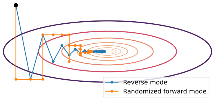
图 8.12：随机化前向模式梯度估计量只需前向传播，但其方差很高，在维数较高时尤甚。Figure 8.12: The randomized forward-mode gradient estimator only requires forward passes, but it suffers from high variance, even more so in high dimension.

8.8 小结8.8 Summary

•

计算机程序可以视为有向无环图：节点对应程序中各中间运算的输出，边则表示当前运算对先前运算的依赖关系。Computer programs can be seen as directed acyclic graphs, where nodes correspond to the output of intermediate operations in the program, and edges represent the dependencies of current operations on past operations.
•

函数 $f\colon\mathbb{R}^{P}\to\mathbb{R}^{M}$ 的自动微分（autodiff）主要有两种模式：前向模式与反向模式。Automatic differentiation (autodiff) for a function $f\colon\mathbb{R}^{P}\to\mathbb{R}^{M}$ has two main modes: forward mode and reverse mode.
•

前向模式：i）使用 JVP；ii）每次构造雅可比矩阵的一列；iii）对高瘦的雅可比矩阵（ $M\geq P$ ）高效；iv）无需存储中间计算。The forward mode: i) uses JVPs, ii) builds the Jacobian one column at a time, iii) is efficient for tall Jacobians ( $M\geq P$ ), iv) need not store intermediate computations.
•

反向模式：i）使用 VJP；ii）每次构造雅可比矩阵的一行；iii）对宽雅可比矩阵（ $P\geq M$ ）高效；iv）需要存储中间计算，才能达到计算上的最优性。The reverse mode: i) uses VJPs, ii) builds the Jacobian one row at a time, iii) is efficient for wide Jacobians ( $P\geq M$ ), iv) needs to store intermediate computations, in order to be computationally optimal.
•

为了以计算效率换取更好的内存效率，我们可以使用检查点技术。To trade computational efficiency for better memory efficiency, we can use checkpointing techniques.
•

使用反向模式计算函数 $f\colon\mathbb{R}^{P}\to\mathbb{R}$ 的梯度的复杂度，至多比求值该函数本身大一个常数倍。这就是算术电路中的 Baur-Strassen 定理。这一惊人的结果是现代机器学习的支柱之一。The complexity of computing the gradient of a function $f\colon\mathbb{R}^{P}\to\mathbb{R}$ using the reverse mode is at most a constant time bigger than that of evaluating the function itself. This is the Baur-Strassen theorem, in arithmetic circuits. This astonishing result is one of the pillars of modern machine learning.

第 8 章 自动微分Chapter 8 Automatic differentiation

8.1 计算链8.1 Computation chains

雅可比矩阵Jacobian matrix

8.1.1 前向模式Forward-mode

计算复杂度Computational complexity

内存占用Memory usage

8.1.2 反向模式Reverse-mode

计算复杂性Computational complexity

内存占用Memory usage

函数求值与 VJP 求值相解耦Decoupled function and VJP evaluations

例 8.1.1（参数固定的多层感知机）。Example 8.1.1 (Multilayer perceptron with fixed parameters ).

8.1.3 计算完整雅可比矩阵的复杂度Complexity of computing entire Jacobians

前向模式自动微分的复杂度Complexity of forward-mode autodiff

反向模式自动微分的复杂度Complexity of reverse-mode autodiff

何时应当使用前向模式自动微分，何时又该使用反向模式自动微分？When to use forward-mode vs. reverse-mode autodiff?

8.2 前馈网络8.2 Feedforward networks

8.2.1 计算伴随Computing the adjoint

8.2.2 计算梯度Computing the gradient

8.3 计算图8.3 Computation graphs

8.3.1 前向模式Forward mode

8.3.2 反向模式Reverse mode

实现Implementation

例 8.3.1（前向模式与反向模式的示例）Example 8.3.1 (Example of forward and reverse modes).

8.3.3 复杂度与 Baur-Strassen 定理Complexity, the Baur-Strassen theorem

命题 8.3.2（Baur-Strassen 定理）Proposition 8.3.2 (Baur-Strassen’s theorem).

8.4 实现8.4 Implementation

8.4.1 基本函数Primitive functions

8.4.2 函数复合下的封闭性Closure under function composition

8.4.3 JVP 与 VJP 的示例Examples of JVPs and VJPs

例 8.4.1（线性函数的 JVP 与 VJP）。Example 8.4.1 (JVP and VJP of linear functions).

例 8.4.2（可分离函数的 JVP 与 VJP）。Example 8.4.2 (JVP and VJP of separable function).

8.4.4 自动线性转置Automatic linear transposition

例 8.4.3（“点积”的自动转置）。Example 8.4.3 (Automatic transpose of “dot”).

8.5 检查点8.5 Checkpointing

两个极端情形下的计算复杂度与内存复杂度Computational and memory complexities at two extremes

8.5.1 递归折半Recursive halving

8.5.2 动态规划Dynamic programming

解析公式Analytical formula

8.5.3 在线检查点Online checkpointing

8.6 可逆层8.6 Reversible layers

8.6.1 一般情形General case

8.6.2 正交归一 JVP 的情形Case of orthonormal JVPs

8.7 随机化前向模式梯度估计量8.7 Randomized forward-mode gradient estimator

命题 8.7.1（梯度的无偏前向模式估计量）。Proposition 8.7.1 (Unbiased forward-mode estimator of the gradient).

8.8 小结8.8 Summary

第 8 章自动微分Chapter 8 Automatic differentiation