目录数据结构

第 6 章 数据结构Chapter 6 Data structures

在计算机科学中,数据结构是组织、存储和访问数据的一种专门格式。在数学上,数据结构构成所谓的代数结构:它由一个集合以及作用于该集合的函数组成。本章讨论如何将数据结构融入可微程序,重点放在列表与字典上。In computer science, a data structure is a specialized format for organizing, storing and accessing data. Mathematically, a data structure forms a so-called algebraic structure: it consists of a set and the functions to operate on that set. In this chapter, we review how to incorporate data structures into differentiable programs, with a focus on lists and dictionaries.

6.1 列表6.1 Lists

列表是元素的有序序列。这里只考虑所有元素都属于同一取值空间 V\mathcal{V} 的列表。形式上,我们把长度为 KK、取值于 V\mathcal{V} 的列表记作一个 KK 元组A list is an ordered sequence of elements. We restrict ourselves to lists whose elements all belong to the same value space V\mathcal{V}. Formally, we denote a list of fixed length KK with values in V\mathcal{V} by a KK-tuple

l:=(l1,…,lK)∈LK(V){\bm{l}}\coloneqq({\bm{l}}_{1},\dots,{\bm{l}}_{K})\in\mathcal{L}_{K}(\mathcal{V})

其中各 li∈V{\bm{l}}_{i}\in\mathcal{V},并且where each li∈V{\bm{l}}_{i}\in\mathcal{V} and where

LK(V):=VK=V×⋯×V⏟K times.\mathcal{L}_{K}(\mathcal{V})\coloneqq\mathcal{V}^{K}=\underbrace{\mathcal{V}\times\dots\times\mathcal{V}}_{K\text{ times}}.

6.1.1 基本操作Basic operations

取值Getting values

我们先介绍如何从列表 l∈LK(V){\bm{l}}\in\mathcal{L}_{K}(\mathcal{V}) 中取出值。定义函数 list.get ⁣:LK(V)×[K]→V\mathrm{list.get}\colon\mathcal{L}_{K}(\mathcal{V})\times[K]\to\mathcal{V} 为We first present how to retrieve values from a list l∈LK(V){\bm{l}}\in\mathcal{L}_{K}(\mathcal{V}). We define the function list.get ⁣:LK(V)×[K]→V\mathrm{list.get}\colon\mathcal{L}_{K}(\mathcal{V})\times[K]\to\mathcal{V} as

list.get(l,i):=li.\mathrm{list.get}({\bm{l}},i)\coloneqq{\bm{l}}_{i}.

该函数关于 l∈LK(V){\bm{l}}\in\mathcal{L}_{K}(\mathcal{V}) 连续且可微,但关于 i∈[K]i\in[K] 不可微,因为后者是离散变量。在 V=R\mathcal{V}=\mathbb{R} 的特殊情形下,LK(V)\mathcal{L}_{K}(\mathcal{V}) 等价于 RK\mathbb{R}^{K},因此可以写成The function is continuous and differentiable in l∈LK(V){\bm{l}}\in\mathcal{L}_{K}(\mathcal{V}) but not in i∈[K]i\in[K], as it is a discrete variable. In the particular case V=R\mathcal{V}=\mathbb{R}, LK(V)\mathcal{L}_{K}(\mathcal{V}) is equivalent to RK\mathbb{R}^{K} and we can therefore write

list.get(l,i)=⟨l,ei⟩,\mathrm{list.get}({\bm{l}},i)=\langle{\bm{l}},{\bm{e}}_{i}\rangle,

其中,{e1,…,eK}\{{\bm{e}}_{1},\dots,{\bm{e}}_{K}\} 是 RK\mathbb{R}^{K} 的标准基。where {e1,…,eK}\{{\bm{e}}_{1},\dots,{\bm{e}}_{K}\} is the standard basis of RK\mathbb{R}^{K}.

设置取值Setting values

接下来,我们介绍如何替换列表 l∈LK(V){\bm{l}}\in\mathcal{L}_{K}(\mathcal{V}) 中的取值。我们定义函数 list.set ⁣:LK(V)×[K]×V→LK(V)\mathrm{list.set}\colon\mathcal{L}_{K}(\mathcal{V})\times[K]\times\mathcal{V}\to\mathcal{L}_{K}(\mathcal{V}) 为We now present how to replace values from a list l∈LK(V){\bm{l}}\in\mathcal{L}_{K}(\mathcal{V}). We define the function list.set ⁣:LK(V)×[K]×V→LK(V)\mathrm{list.set}\colon\mathcal{L}_{K}(\mathcal{V})\times[K]\times\mathcal{V}\to\mathcal{L}_{K}(\mathcal{V}) as

[list.set(l,i,v)]j:={v if i=jlj if i≠j,[\mathrm{list.set}({\bm{l}},i,{\bm{v}})]_{j}\coloneqq\begin{cases}{\bm{v}}&\text{ if }i=j\\ {\bm{l}}_{j}&\text{ if }i\neq j\end{cases},

其中 j∈[K]j\in[K]。本着函数式编程的精神,即使只改动了一个元素,该函数返回的也是整个新列表。同样,该函数关于 l∈LK(V){\bm{l}}\in\mathcal{L}_{K}(\mathcal{V}) 与 v∈V{\bm{v}}\in\mathcal{V} 连续且可微,关于 i∈[K]i\in[K] 则不可微。在 V=R\mathcal{V}=\mathbb{R} 的特殊情形下,对于给定列表 l=(l1,…,lK){\bm{l}}=(l_{1},\dots,l_{K}),可以通过下式设置值 v∈Rv\in\mathbb{R}:for j∈[K]j\in[K]. In the functional programming spirit, the function returns the whole new list, even though a single element has been modified. Again, the function is continuous and differentiable in l∈LK(V){\bm{l}}\in\mathcal{L}_{K}(\mathcal{V}) and v∈V{\bm{v}}\in\mathcal{V} but not in i∈[K]i\in[K]. In the particular case V=R\mathcal{V}=\mathbb{R}, given a list l=(l1,…,lK){\bm{l}}=(l_{1},\dots,l_{K}), we can set the value v∈Rv\in\mathbb{R} by

list.set(l,i,v)=l+(v−li)ei.\mathrm{list.set}({\bm{l}},i,v)={\bm{l}}+(v-l_{i}){\bm{e}}_{i}.

也就是说,我们在 l{\bm{l}} 中位置 i∈[K]i\in[K] 处减去旧值 lil_{i},再加上新值 vv。That is, we subtract the old value lil_{i} and add the new value vv at the location i∈[K]i\in[K] in l{\bm{l}}.

实现Implementation

定长列表可以用数组实现,从而支持对各元素的 O(1)O(1) 随机访问。数组在硬件上的对应物是随机存取存储器(RAM),其中内存可按地址(位置)取用。A fixed-length list can be implemented as an array, which enables O(1)O(1) random access to individual elements. The hardware counterpart of an array is random access memory (RAM), in which memory can be retrieved by address (location).

6.1.2 变长列表上的操作Operations on variable-length lists

此前,我们关注的都是长度为 KK 的定长列表。现在我们转而讨论变长列表,它的大小可以随时间缩小或增大。除了 list.get\mathrm{list.get} 和 list.set\mathrm{list.set} 函数之外,它还支持能够改变列表大小的函数。So far, we focused on lists of fixed length KK. We now turn our attention to variable-length lists, whose size can decrease or increase over time. In addition to the list.get\mathrm{list.get} and list.set\mathrm{list.set} functions, they support functions that can change the size of a list.

初始化列表Initializing lists

为了初始化列表,我们定义 list.init ⁣:V→L1(V)\mathrm{list.init}\colon\mathcal{V}\to\mathcal{L}_{1}(\mathcal{V}) 为In order to initialize a list, we define list.init ⁣:V→L1(V)\mathrm{list.init}\colon\mathcal{V}\to\mathcal{L}_{1}(\mathcal{V}) as

list.init(v):=(v),\mathrm{list.init}({\bm{v}})\coloneqq({\bm{v}}),

其中,我们用 (v)({\bm{v}}) 表示一个 11 元组。where we used (v)({\bm{v}}) to denote a 11-tuple.

压入取值Pushing values

为了向左侧或右侧添加新值,我们定义 list.pushLeft ⁣:LK(V)×V→LK+1(V)\mathrm{list.pushLeft}\colon\mathcal{L}_{K}(\mathcal{V})\times\mathcal{V}\to\mathcal{L}_{K+1}(\mathcal{V}) 为In order to add new values either to the left or to the right, we define list.pushLeft ⁣:LK(V)×V→LK+1(V)\mathrm{list.pushLeft}\colon\mathcal{L}_{K}(\mathcal{V})\times\mathcal{V}\to\mathcal{L}_{K+1}(\mathcal{V}) as

list.pushLeft(l,v):=(v,l1,…,lK).\mathrm{list.pushLeft}({\bm{l}},{\bm{v}})\coloneqq({\bm{v}},{\bm{l}}_{1},\dots,{\bm{l}}_{K}).

以及 list.pushRight ⁣:LK(V)×V→LK+1(V)\mathrm{list.pushRight}\colon\mathcal{L}_{K}(\mathcal{V})\times\mathcal{V}\to\mathcal{L}_{K+1}(\mathcal{V}) 为and list.pushRight ⁣:LK(V)×V→LK+1(V)\mathrm{list.pushRight}\colon\mathcal{L}_{K}(\mathcal{V})\times\mathcal{V}\to\mathcal{L}_{K+1}(\mathcal{V}) as

list.pushRight(l,v):=(l1,…,lK,v).\mathrm{list.pushRight}({\bm{l}},{\bm{v}})\coloneqq({\bm{l}}_{1},\dots,{\bm{l}}_{K},{\bm{v}}).

弹出取值Popping values

为了从左侧或右侧移除值,我们定义 list.popLeft ⁣:LK(V)→LK−1(V)×V\mathrm{list.popLeft}\colon\mathcal{L}_{K}(\mathcal{V})\to\mathcal{L}_{K-1}(\mathcal{V})\times\mathcal{V} 为In order to remove values either from the left or from the right, we define list.popLeft ⁣:LK(V)→LK−1(V)×V\mathrm{list.popLeft}\colon\mathcal{L}_{K}(\mathcal{V})\to\mathcal{L}_{K-1}(\mathcal{V})\times\mathcal{V} as

list.popLeft(l):=(l2,…,lK),l1\mathrm{list.popLeft}({\bm{l}})\coloneqq({\bm{l}}_{2},\dots,{\bm{l}}_{K}),{\bm{l}}_{1}

以及 list.popRight ⁣:LK(V)→LK−1(V)×V\mathrm{list.popRight}\colon\mathcal{L}_{K}(\mathcal{V})\to\mathcal{L}_{K-1}(\mathcal{V})\times\mathcal{V} 为and list.popRight ⁣:LK(V)→LK−1(V)×V\mathrm{list.popRight}\colon\mathcal{L}_{K}(\mathcal{V})\to\mathcal{L}_{K-1}(\mathcal{V})\times\mathcal{V} as

list.popRight(l):=(l1,…,lK−1),lK.\mathrm{list.popRight}({\bm{l}})\coloneqq({\bm{l}}_{1},\dots,{\bm{l}}_{K-1}),{\bm{l}}_{K}.

集合 L0(V)\mathcal{L}_{0}(\mathcal{V}) 是只含空列表的单元素集。The set L0(V)\mathcal{L}_{0}(\mathcal{V}) is a singleton which contains the empty list.

插入取值Inserting values

pushLeft 与 pushRight 函数只能分别把值插入列表开头和末尾。现在我们研究 insert 函数,其目标是在任意位置添加新值,并将所有值右移,使列表大小增加 11。我们定义函数 list.insert:LK(V)×[K+1]×V→LK+1(V)\mathrm{list.insert}:\mathcal{L}_{K}(\mathcal{V})\times[K+1]\times\mathcal{V}\rightarrow\mathcal{L}_{K+1}(\mathcal{V}) 为The pushLeft and pushRight functions can only insert values at the beginning and at the end of a list, respectively. We now study the insert function, whose goal is to be able to add a new value at an arbitrary location, shifting all values to the right and increasing the list size by 11. We define the function list.insert:LK(V)×[K+1]×V→LK+1(V)\mathrm{list.insert}:\mathcal{L}_{K}(\mathcal{V})\times[K+1]\times\mathcal{V}\rightarrow\mathcal{L}_{K+1}(\mathcal{V}) as

[list.insert(l,i,v)]j:={ljif j<ivif j=ilj−1if j>i,[\mathrm{list.insert}({\bm{l}},i,{\bm{v}})]_{j}\coloneqq\begin{cases}{\bm{l}}_{j}&\text{if}\ j<i\\ {\bm{v}}&\text{if}\ j=i\\ {\bm{l}}_{j-1}&\text{if}\ j>i\end{cases},

其中 j∈[K+1]j\in[K+1]。与 list.set\mathrm{list.set} 函数一样,list.insert\mathrm{list.insert} 关于 l{\bm{l}} 与 v{\bm{v}} 显然是连续且可微的,关于 ii 则不可微,因为后者是离散变量。作为特例,我们自然得到for j∈[K+1]j\in[K+1]. As for the list.set\mathrm{list.set} function, list.insert\mathrm{list.insert} is readily continuous and differentiable in l{\bm{l}} and v{\bm{v}}, but not in ii, as it is a discrete variable. As special cases, we naturally recover

list.insert(l,1,v)\displaystyle\mathrm{list.insert}({\bm{l}},1,{\bm{v}}) =list.pushLeft(l,v),\displaystyle=\mathrm{list.pushLeft}({\bm{l}},{\bm{v}}),
list.insert(l,K+1,v)\displaystyle\mathrm{list.insert}({\bm{l}},K+1,{\bm{v}}) =list.pushRight(l,v).\displaystyle=\mathrm{list.pushRight}({\bm{l}},{\bm{v}}).

可微性Differentiability

对于 list.init\mathrm{list.init}、list.push\mathrm{list.push} 和 list.pop\mathrm{list.pop} 函数,其关于自变量的连续性与可微性都是显然的(无需连续松弛)。至于 list.set\mathrm{list.set} 函数,list.insert\mathrm{list.insert} 函数关于 l{\bm{l}} 和 v{\bm{v}} 连续且可微,但关于 ii 则不然。The list.init\mathrm{list.init}, list.push\mathrm{list.push} and list.pop\mathrm{list.pop} functions are readily continuous and differentiable with respect to their arguments (a continuous relaxation is not needed). As for the list.set\mathrm{list.set} function, the list.insert\mathrm{list.insert} function is continuous and differentiable in l{\bm{l}} and v{\bm{v}}, but not in ii.

实现Implementation

在底层,变长列表可以实现为链表或动态数组。链表提供 O(K)O(K) 随机访问,而动态数组允许 O(1)O(1) 随机访问,代价是需要进行内存重分配。Under the hood, a variable-length list can be implemented as a linked list or as a dynamic array. A linked list gives O(K)O(K) random access while a dynamic array allows O(1)O(1) random access, at the cost of memory reallocations.

栈与队列Stacks and queues

list.pushRight\mathrm{list.pushRight} 和 list.popRight\mathrm{list.popRight} 函数可用于实现栈(后进先出,又称 LIFO 行为)。list.pushLeft\mathrm{list.pushLeft} 和 list.popRight\mathrm{list.popRight} 函数可用于实现队列(先进先出,又称 FIFO 行为)。The list.pushRight\mathrm{list.pushRight} and list.popRight\mathrm{list.popRight} functions can be used to implement a stack (last in first out a.k.a. LIFO behavior). The list.pushLeft\mathrm{list.pushLeft} and list.popRight\mathrm{list.popRight} functions can be used to implement a queue (first in first out a.k.a. FIFO behavior).

6.1.3 使用软索引的连续松弛Continuous relaxations using soft indexing

获取取值Getting values

为了能够关于索引对 list.get\mathrm{list.get} 求导,一个自然的想法是用分布 πi∈△K{\bm{\pi}}_{i}\in\triangle^{K} 替换整数索引 i∈[K]i\in[K],我们可以将其解释为软索引。于是整数索引 i∈[K]i\in[K] 等价于 delta 分布 πi∈{e1,…,eK}{\bm{\pi}}_{i}\in\{{\bm{e}}_{1},\dots,{\bm{e}}_{K}\}。我们将连续松弛 list.softGet ⁣:LK(V)×△K→conv⁡(V)\mathrm{list.softGet}\colon\mathcal{L}_{K}(\mathcal{V})\times\triangle^{K}\to\conv(\mathcal{V}) 定义为In order to be able to differentiate list.get\mathrm{list.get} w.r.t. indexing, a natural idea is to replace the integer index i∈[K]i\in[K] by a distribution πi∈△K{\bm{\pi}}_{i}\in\triangle^{K}, which we can interpret as a soft index. An integer index i∈[K]i\in[K] is then equivalent to a delta distribution πi∈{e1,…,eK}{\bm{\pi}}_{i}\in\{{\bm{e}}_{1},\dots,{\bm{e}}_{K}\}. We define the continuous relaxation list.softGet ⁣:LK(V)×△K→conv⁡(V)\mathrm{list.softGet}\colon\mathcal{L}_{K}(\mathcal{V})\times\triangle^{K}\to\conv(\mathcal{V}) as

list.softGet(l,πi)\displaystyle\mathrm{list.softGet}({\bm{l}},{\bm{\pi}}_{i}) :=∑j=1Kπi,jlj\displaystyle\coloneqq\sum_{j=1}^{K}\pi_{i,j}{\bm{l}}_{j}
=cond(πi,l1,…,lK)\displaystyle=\mathrm{cond}({\bm{\pi}}_{i},{\bm{l}}_{1},\dots,{\bm{l}}_{K})
=EI∼Categorical(πi)[lI],\displaystyle=\mathbb{E}_{I\sim\mathrm{Categorical}({\bm{\pi}}_{i})}[{\bm{l}}_{I}],

其中 cond\mathrm{cond} 已在第 5.7 节中研究。在 V=R\mathcal{V}=\mathbb{R} 的特殊情形下,可得where cond\mathrm{cond} is studied in Section 5.7. In the particular case V=R\mathcal{V}=\mathbb{R}, we obtain

list.softGet(l,i)=⟨l,πi⟩.\mathrm{list.softGet}({\bm{l}},i)=\langle{\bm{l}},{\bm{\pi}}_{i}\rangle.

这一点如图 6.1 所示。This is illustrated in Fig. 6.1.

分布 πi=(πi,1,…,πi,K){\bm{\pi}}_{i}=(\pi_{i,1},\dots,\pi_{i,K}) 的选择编码了各元素 (l1,…,lK)({\bm{l}}_{1},\dots,{\bm{l}}_{K}) 关于 li{\bm{l}}_{i} 的重要性。如果我们认为 ∣i−j∣|i-j| 越小,li{\bm{l}}_{i} 与 lj{\bm{l}}_{j} 的相关性就越强,那么定义以 ii 为中心的分布(即分布的众数在 ii 处取得)就是合理的。例如,将范围限制在邻居 li−1{\bm{l}}_{i-1} 和 li+1{\bm{l}}_{i+1}(即大小为 11 的窗口),我们可以定义稀疏分布The choice of the distribution πi=(πi,1,…,πi,K){\bm{\pi}}_{i}=(\pi_{i,1},\dots,\pi_{i,K}) encodes the importance of the elements (l1,…,lK)({\bm{l}}_{1},\dots,{\bm{l}}_{K}) w.r.t. li{\bm{l}}_{i}. If we consider that the smaller ∣i−j∣|i-j| is, the more related li{\bm{l}}_{i} and lj{\bm{l}}_{j} are, then it makes sense to define a distribution centered around ii (i.e., such that the mode of the distribution is achieved at ii). For example, limiting ourselves to the neighbors li−1{\bm{l}}_{i-1} and li+1{\bm{l}}_{i+1} (i.e., a window of size 11), we can define the sparse distribution

πi:=14⋅ei−1+12ei+14⋅ei+1∈△K.{\bm{\pi}}_{i}\coloneqq\frac{1}{4}\cdot{\bm{e}}_{i-1}+\frac{1}{2}{\bm{e}}_{i}+\frac{1}{4}\cdot{\bm{e}}_{i+1}\in\triangle^{K}.

在这种特殊情形下,list.get\mathrm{list.get} 函数的连续松弛可以表示为离散卷积,In this particular case, the continuous relaxation of the list.get\mathrm{list.get} function can then be expressed as a discrete convolution,

list.softGet(l,πi)=(list.get(l,⋅)∗κ)(i)=∑j=−∞∞list.get(l,i−j)κ(j),\mathrm{list.softGet}({\bm{l}},{\bm{\pi}}_{i})=\left(\mathrm{list.get}({\bm{l}},\cdot)\ast\kappa\right)(i)=\sum_{j=-\infty}^{\infty}\mathrm{list.get}({\bm{l}},i-j)\kappa(j),

其中 κ(−1):=14\kappa(-1)\coloneqq\frac{1}{4}、κ(1):=14\kappa(1)\coloneqq\frac{1}{4}、κ(0):=12\kappa(0)\coloneqq\frac{1}{2},且对于 j∉{−1,0,1}j\not\in\{-1,0,1\} 有 κ(j):=0\kappa(j)\coloneqq 0。假设 V=RM\mathcal{V}=\mathbb{R}^{M},则 list.softGet\mathrm{list.softGet} 的计算复杂度为 O(M⋅∣supp(πi)∣)O(M\cdot|\mathrm{supp}({\bm{\pi}}_{i})|)。where κ(−1):=14\kappa(-1)\coloneqq\frac{1}{4}, κ(1):=14\kappa(1)\coloneqq\frac{1}{4}, κ(0):=12\kappa(0)\coloneqq\frac{1}{2}, and κ(j):=0\kappa(j)\coloneqq 0 for j∉{−1,0,1}j\not\in\{-1,0,1\}. Assuming V=RM\mathcal{V}=\mathbb{R}^{M}, the computational complexity of list.softGet\mathrm{list.softGet} is O(M⋅∣supp(πi)∣)O(M\cdot|\mathrm{supp}({\bm{\pi}}_{i})|).

图 6.1:list.get(l,i)\mathrm{list.get}({\bm{l}},i) 函数在 l{\bm{l}} 上连续且可微,但在 ii 上不可微。其松弛 list.softGet(l,πi)\mathrm{list.softGet}({\bm{l}},{\bm{\pi}}_{i}) 在 l{\bm{l}} 和 πi{\bm{\pi}}_{i} 上均可微。当 V=R\mathcal{V}=\mathbb{R} 时,list.softGet(l,πi)\mathrm{list.softGet}({\bm{l}},{\bm{\pi}}_{i}) 可看作是在列表 l{\bm{l}} 与概率分布 πi{\bm{\pi}}_{i} 之间取内积,而非与 delta 分布(标准向量)ei{\bm{e}}_{i} 取内积。Figure 6.1: The list.get(l,i)\mathrm{list.get}({\bm{l}},i) function is continuous and differentiable in l{\bm{l}} but not in ii. Its relaxation list.softGet(l,πi)\mathrm{list.softGet}({\bm{l}},{\bm{\pi}}_{i}) is differentiable in both l{\bm{l}} and πi{\bm{\pi}}_{i}. When V=R\mathcal{V}=\mathbb{R}, list.softGet(l,πi)\mathrm{list.softGet}({\bm{l}},{\bm{\pi}}_{i}) can be seen as taking the inner product between the list l{\bm{l}} and the probability distribution πi{\bm{\pi}}_{i}, instead of the delta distribution (canonical vector) ei{\bm{e}}_{i}.

设置取值Setting values

为了对索引求导,我们可以将连续松弛 list.softSet ⁣:LK(V)×△K×V→LK(conv⁡(V))\mathrm{list.softSet}\colon\mathcal{L}_{K}(\mathcal{V})\times\triangle^{K}\times\mathcal{V}\to\mathcal{L}_{K}(\conv(\mathcal{V})) 定义为To differentiate w.r.t. indexing, we can define the continuous relaxation list.softSet ⁣:LK(V)×△K×V→LK(conv⁡(V))\mathrm{list.softSet}\colon\mathcal{L}_{K}(\mathcal{V})\times\triangle^{K}\times\mathcal{V}\to\mathcal{L}_{K}(\conv(\mathcal{V})) as

[list.softSet(l,πi,v)]j\displaystyle\left[\mathrm{list.softSet}({\bm{l}},{\bm{\pi}}_{i},{\bm{v}})\right]_{j} :=E[list.set(l,I,v)]j\displaystyle\coloneqq\mathbb{E}[\mathrm{list.set}({\bm{l}},I,{\bm{v}})]_{j}
=P(I=j)v+P(I≠j)lj\displaystyle=\mathbb{P}(I=j){\bm{v}}+\mathbb{P}(I\neq j){\bm{l}}_{j}
=πi,jv+(1−πi,j)lj,\displaystyle=\pi_{i,j}{\bm{v}}+(1-\pi_{i,j}){\bm{l}}_{j},

其中 j∈[K]j\in[K],且 I∼Categorical(πi)I\sim\mathrm{Categorical}({\bm{\pi}}_{i})。等价地,可以写为where j∈[K]j\in[K] and I∼Categorical(πi)I\sim\mathrm{Categorical}({\bm{\pi}}_{i}). Equivalently, we can write

list.softSet(l,πi,v)\displaystyle\mathrm{list.softSet}({\bm{l}},{\bm{\pi}}_{i},{\bm{v}}) =(πi,1v+(1−πi,1)l1,…,πi,Kv+(1−πi,K)lK)\displaystyle=(\pi_{i,1}{\bm{v}}+(1-\pi_{i,1}){\bm{l}}_{1},\dots,\pi_{i,K}{\bm{v}}+(1-\pi_{i,K}){\bm{l}}_{K})
=(ifelse(πi,1,v,l1),…,ifelse(πi,K,v,lK)),\displaystyle=(\mathrm{ifelse}(\pi_{i,1},{\bm{v}},{\bm{l}}_{1}),\dots,\mathrm{ifelse}(\pi_{i,K},{\bm{v}},{\bm{l}}_{K})),

其中 ifelse\mathrm{ifelse} 已在第 5.6 节中研究。由于where ifelse\mathrm{ifelse} is studied in Section 5.6. Since

ifelse(π,u1,u0)=EI∼Bernoulli(π)[uI],\mathrm{ifelse}(\pi,{\bm{u}}_{1},{\bm{u}}_{0})=\mathbb{E}_{I\sim\mathrm{Bernoulli}(\pi)}[{\bm{u}}_{I}],

这一松弛相当于使用逐元素期望。因此,list.softSet\mathrm{list.softSet} 输出的列表取值于 conv⁡(V)\conv(\mathcal{V}) 而非 V\mathcal{V}。不过要注意,当 V=RM\mathcal{V}=\mathbb{R}^{M} 时,也有 conv⁡(V)=RM\conv(\mathcal{V})=\mathbb{R}^{M}。this relaxation amounts to using an element-wise expectation. As a result, the list output by list.softSet\mathrm{list.softSet} takes values in conv⁡(V)\conv(\mathcal{V}) instead of V\mathcal{V}. Note however that when V=RM\mathcal{V}=\mathbb{R}^{M}, then conv⁡(V)=RM\conv(\mathcal{V})=\mathbb{R}^{M} as well.

插入取值Inserting values

为了关于索引对取值插入求导,我们可以将连续松弛 list.softInsert ⁣:LK(V)×△K+1×V→LK+1(conv⁡(V))\mathrm{list.softInsert}\colon\mathcal{L}_{K}(\mathcal{V})\times\triangle^{K+1}\times\mathcal{V}\to\mathcal{L}_{K+1}(\conv(\mathcal{V})) 定义为To differentiate value insertion w.r.t. indexing, we can define the continuous relaxation list.softInsert ⁣:LK(V)×△K+1×V→LK+1(conv⁡(V))\mathrm{list.softInsert}\colon\mathcal{L}_{K}(\mathcal{V})\times\triangle^{K+1}\times\mathcal{V}\to\mathcal{L}_{K+1}(\conv(\mathcal{V})) as

[list.softInsert(l,πi,v)]j\displaystyle[\mathrm{list.softInsert}({\bm{l}},{\bm{\pi}}_{i},{\bm{v}})]_{j} :=E[list.insert(l,I,v)]\displaystyle\coloneqq\mathbb{E}[\mathrm{list.insert}({\bm{l}},I,{\bm{v}})]
=P(I>j)lj+P(I=j)v+P(I<j)lj−1,\displaystyle=\mathbb{P}(I>j){\bm{l}}_{j}+\mathbb{P}(I=j){\bm{v}}+\mathbb{P}(I<j){\bm{l}}_{j-1},

其中 I∼Categorical(πi)I\sim\mathrm{Categorical}({\bm{\pi}}_{i})。对于 j∈[K+1]j\in[K+1],三个必要的概率很容易通过下式计算where I∼Categorical(πi)I\sim\mathrm{Categorical}({\bm{\pi}}_{i}). The three necessary probabilities can easily be calculated for j∈[K+1]j\in[K+1] by

P(I>j)\displaystyle\mathbb{P}(I>j) ={0 if j=K+1∑k=j+1K+1πi,k otherwise \displaystyle=\begin{cases}0&\text{ if }j=K+1\\ \sum_{k=j+1}^{K+1}\pi_{i,k}&\text{ otherwise }\end{cases}
P(I=j)\displaystyle\mathbb{P}(I=j) =πi,j\displaystyle=\pi_{i,j}\quad
P(I<j)\displaystyle\mathbb{P}(I<j) ={0 if j=1∑k=1j−1πi,k otherwise .\displaystyle=\begin{cases}0&\text{ if }j=1\\ \sum_{k=1}^{j-1}\pi_{i,k}&\text{ otherwise }\end{cases}.

多维索引Multi-dimensional indexing

在多维列表(数组或张量)中,列表 l∈LK1,…,KT(V){\bm{l}}\in\mathcal{L}_{K_{1},\dots,K_{T}}(\mathcal{V}) 的每个元素 li∈V{\bm{l}}_{\bm{i}}\in\mathcal{V} 现在都可以用多元整数 i=(i1,…,iT)∈[K1]×⋯×[KT]{\bm{i}}=(i_{1},\dots,i_{T})\in[K_{1}]\times\dots\times[K_{T}] 来索引,其中 T∈NT\in\mathbb{N} 是 l{\bm{l}} 的轴数。我们总是可以通过将多维索引 i∈[K1]×⋯×[KT]{\bm{i}}\in[K_{1}]\times\dots\times[K_{T}] 替换为展平索引 i∈[K1…KT]i\in[K_{1}\dots K_{T}],把多维列表展平为一维列表;反过来,将展平的一维数组转换为多维数组也是可行的。因此,对于 K:=K1…KTK\coloneqq K_{1}\dots K_{T},[K][K] 与 [K1]×⋯×[KT][K_{1}]\times\dots\times[K_{T}] 之间存在双射。In multi-dimensional lists (arrays or tensors), each element li∈V{\bm{l}}_{\bm{i}}\in\mathcal{V} of a list l∈LK1,…,KT(V){\bm{l}}\in\mathcal{L}_{K_{1},\dots,K_{T}}(\mathcal{V}) can now be indexed by a multivariate integer i=(i1,…,iT)∈[K1]×⋯×[KT]{\bm{i}}=(i_{1},\dots,i_{T})\in[K_{1}]\times\dots\times[K_{T}], where T∈NT\in\mathbb{N} is the number of axes of l{\bm{l}}. We can always flatten a multi-dimensional list into a uni-dimensional list by replacing the multi-dimensional index i∈[K1]×⋯×[KT]{\bm{i}}\in[K_{1}]\times\dots\times[K_{T}] by a flat index i∈[K1…KT]i\in[K_{1}\dots K_{T}]. The converse operation, converting a flat uni-dimensional array into a multi-dimensional array, is also possible. Therefore, there is a bijection between [K][K] and [K1]×⋯×[KT][K_{1}]\times\dots\times[K_{T}] for K:=K1…KTK\coloneqq K_{1}\dots K_{T}.

这意味着,前文关于一维情形下软索引的讨论可直接推广到多维情形。所需的只是定义一个概率分布 πi∈△K1×⋯×KT{\bm{\pi}}_{\bm{i}}\in\triangle^{K_{1}\times\dots\times K_{T}} 的能力。例如,在处理图像时,我们可以定义一个概率分布,使其概率质量只落在像素 i{\bm{i}} 的相邻像素上,这是图像处理中的标准做法。另一种简单做法是采用各轴概率分布的乘积。This means that the previous discussion on soft indexing in the uni-dimensional setting readily applies to the multi-dimensional setting. All it takes is the ability to define a probability distribution πi∈△K1×⋯×KT{\bm{\pi}}_{\bm{i}}\in\triangle^{K_{1}\times\dots\times K_{T}}. For example, when working with images, we can define a probability distribution putting probability mass only on the neighboring pixels of pixel i{\bm{i}}, a standard approach in image processing. Another simple approach is to use a product of axis-wise probability distributions.

6.2 字典6.2 Dictionaries

字典(又称关联数组或映射)是键—值对的无序列表,其中每个可能的键在列表中最多出现一次。我们将键的集合记为 K\mathcal{K},将值的集合记为 V\mathcal{V}(两者都可能是无穷集)。于是,我们可以定义从 K\mathcal{K} 到 V\mathcal{V} 的、大小为 LL 的字典集合为A dictionary (a.k.a. associative array or map) is an unordered list of key-value pairs, such that each possible key appears at most once in the list. We denote the set of keys by K\mathcal{K} and the set of values by V\mathcal{V} (both being potentially infinite). We can then define the set of dictionaries of size LL from K\mathcal{K} to V\mathcal{V} by

DL(K,V):=LL(K×V)=(K×V)L\mathcal{D}_{L}(\mathcal{K},\mathcal{V})\coloneqq\mathcal{L}_{L}(\mathcal{K}\times\mathcal{V})=(\mathcal{K}\times\mathcal{V})^{L}

而一个这样的字典由and one such dictionary by

d:=((k1,v1),…,(kL,vL))∈DL(K,V).{\bm{d}}\coloneqq(({\bm{k}}_{1},{\bm{v}}_{1}),\dots,({\bm{k}}_{L},{\bm{v}}_{L}))\in\mathcal{D}_{L}(\mathcal{K},\mathcal{V}).

6.2.1 基本操作Basic operations

获取取值Getting values

dict.get\mathrm{dict.get} 函数的目标是取回与某个键相关联的值,前提是字典包含该键。形式上,我们将 dict.get ⁣:DL(K,V)×K→V∪{∞}\mathrm{dict.get}\colon\mathcal{D}_{L}(\mathcal{K},\mathcal{V})\times\mathcal{K}\to\mathcal{V}\cup\{\infty\} 函数定义为The goal of the dict.get\mathrm{dict.get} function is to retrieve the value associated with a key, assuming that the dictionary contains this key. Formally, we define the dict.get ⁣:DL(K,V)×K→V∪{∞}\mathrm{dict.get}\colon\mathcal{D}_{L}(\mathcal{K},\mathcal{V})\times\mathcal{K}\to\mathcal{V}\cup\{\infty\} function as

dict.get(d,k):={vi if ∃i∈[L] s.t. k=ki∞ if k∉{k1,…,kL}.\mathrm{dict.get}({\bm{d}},{\bm{k}})\coloneqq\begin{cases}{\bm{v}}_{i}&\text{ if }\exists i\in[L]\text{ s.t. }{\bm{k}}={\bm{k}}_{i}\\ \infty&\text{ if }{\bm{k}}\not\in\{{\bm{k}}_{1},\dots,{\bm{k}}_{L}\}\end{cases}.

该函数关于字典 d{\bm{d}} 连续且可微,但关于键 k{\bm{k}} 则不然。等价地,我们可以将该函数写为The function is continuous and differentiable in the dictionary d{\bm{d}}, but not in the key k{\bm{k}}. Equivalently, we can write the function as

dict.get(d,k):=∑i=1Leq(k,ki)vi∑i=1Leq(k,ki).\displaystyle\mathrm{dict.get}({\bm{d}},{\bm{k}})\coloneqq\frac{\sum_{i=1}^{L}\mathrm{eq}({\bm{k}},{\bm{k}}_{i}){\bm{v}}_{i}}{\sum_{i=1}^{L}\mathrm{eq}({\bm{k}},{\bm{k}}_{i})}.

分母体现了这样一个事实:若字典 d{\bm{d}} 中没有键与键 k{\bm{k}} 相匹配,则该函数无定义。假设 k∈{k1,…,kL}{\bm{k}}\in\{{\bm{k}}_{1},\dots,{\bm{k}}_{L}\} 且 V=RM\mathcal{V}=\mathbb{R}^{M},我们也可以将其写为The denominator encodes the fact that the function is undefined if no key in the dictionary d{\bm{d}} matches the key k{\bm{k}}. Assuming k∈{k1,…,kL}{\bm{k}}\in\{{\bm{k}}_{1},\dots,{\bm{k}}_{L}\} and V=RM\mathcal{V}=\mathbb{R}^{M}, we can also write

dict.get(d,k)=viwherei=arg max⁡j∈[L]∥k−kj∥2,\mathrm{dict.get}({\bm{d}},{\bm{k}})={\bm{v}}_{i}\quad\text{where}\quad i=\argmax_{j\in[L]}\|{\bm{k}}-{\bm{k}}_{j}\|_{2},

这表明,我们可以把 dict.get\mathrm{dict.get} 看作最近邻搜索。which shows that we can see dict.get\mathrm{dict.get} as a nearest neighbor search.

设置取值Setting values

dict.set\mathrm{dict.set} 函数的目标是替换与某个已有键相关联的值。形式上,我们将 dict.set:DL(K,V)×K×V→DL(K,V)\mathrm{dict.set}:\mathcal{D}_{L}(\mathcal{K},\mathcal{V})\times\mathcal{K}\times\mathcal{V}\rightarrow\mathcal{D}_{L}(\mathcal{K},\mathcal{V}) 函数定义为The goal of the dict.set\mathrm{dict.set} function is to replace the value associated with an existing key. Formally, we define the dict.set:DL(K,V)×K×V→DL(K,V)\mathrm{dict.set}:\mathcal{D}_{L}(\mathcal{K},\mathcal{V})\times\mathcal{K}\times\mathcal{V}\rightarrow\mathcal{D}_{L}(\mathcal{K},\mathcal{V}) function as

(dict.set(d,k,v))i:={(ki,v)if ki=k(ki,vi)if ki≠k.(\mathrm{dict.set}({\bm{d}},{\bm{k}},{\bm{v}}))_{i}\coloneqq\begin{cases}({\bm{k}}_{i},{\bm{v}})&\text{if}\ {\bm{k}}_{i}={\bm{k}}\\ ({\bm{k}}_{i},{\bm{v}}_{i})&\text{if}\ {\bm{k}}_{i}\neq{\bm{k}}\end{cases}.

如果字典中没有键与输入键 k{\bm{k}} 相匹配,则该函数保持字典不变。该函数关于 d{\bm{d}} 和 v{\bm{v}} 连续且可微,但关于 k{\bm{k}} 则不然。The function leaves the dictionary unchanged if no key in the dictionary matches the input key k{\bm{k}}. The function is continuous and differentiable in d{\bm{d}} and v{\bm{v}}, but not in k{\bm{k}}.

实现Implementation

尽管我们将字典视为键—值对的列表,但在实践中,字典(又称关联数组)通常使用哈希表或搜索树来实现。字典在硬件上的对应物称为内容寻址存储器(CAM),又称关联存储器。While we view dictionaries as lists of key-value pairs, in practice, a dictionary (a.k.a. associative array) is often implemented using a hash table or search trees. The hardware counterpart of a dictionary is called content-addressable memory (CAM), a.k.a. associative memory.

6.2.2 使用核回归的连续松弛Continuous relaxation using kernel regression
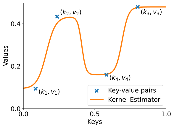
图 6.2:给定一组定义字典 d{\bm{d}} 的键—值对 (ki,vi)∈K×V({\bm{k}}_{i},{\bm{v}}_{i})\in\mathcal{K}\times\mathcal{V},我们可以借助 Nadaraya–Watson 核回归估计从 K\mathcal{K} 到 V\mathcal{V} 的连续映射(此处以 K=V=R\mathcal{K}=\mathcal{V}=\mathbb{R} 为例进行说明)。当键被归一化为单位范数时,这便恢复了 Transformer 中的 softargmax 注意力。Figure 6.2: Given a set of key-value pairs (ki,vi)∈K×V({\bm{k}}_{i},{\bm{v}}_{i})\in\mathcal{K}\times\mathcal{V} defining a dictionary d{\bm{d}}, we can estimate a continuous mapping from K\mathcal{K} to V\mathcal{V} using Nadaraya–Watson kernel regression (here, illustrated with K=V=R\mathcal{K}=\mathcal{V}=\mathbb{R}). When keys are normalized to have unit norm, this recovers softargmax attention from Transformers.

可以将字典视为一个(可能非单射的)函数,它为每个键 v{\bm{v}} 关联一个值 k{\bm{k}}。为得到与字典相关操作的连续松弛,我们可以采用从键到值的映射的概率视角:把键和值视为两个连续随机变量 KK 与 VV。于是,我们可以用 f(v∣k)f({\bm{v}}|{\bm{k}}) 的联合 PDF V∣KV|K 以及 f(k,v)f({\bm{k}},{\bm{v}}) 的边缘 PDF (K,V)(K,V) 来表示 f(k)f({\bm{k}}) 的条件 PDF KK,即A dictionary can be seen as a (potentially non-injective) function that associates a value v{\bm{v}} to each key k{\bm{k}}. To obtain a continuous relaxation of the operations associated to a dictionary, we can adopt a probabilistic perspective of the mapping from keys to values. We can view keys and values as two continuous random variables KK and VV. We can express the conditional PDF f(v∣k)f({\bm{v}}|{\bm{k}}) of V∣KV|K in terms of the joint PDF f(k,v)f({\bm{k}},{\bm{v}}) of (K,V)(K,V) and the marginal PDF f(k)f({\bm{k}}) of KK as

f(v∣k)=f(k,v)f(k).f({\bm{v}}|{\bm{k}})=\frac{f({\bm{k}},{\bm{v}})}{f({\bm{k}})}.

对其积分,我们得到条件期望Integrating, we obtain the conditional expectation

E[V∣K=k]=∫Vf(v∣k)vdv=∫Vf(k,v)f(k)vdv.\displaystyle\mathbb{E}[V|K={\bm{k}}]=\int_{\mathcal{V}}f({\bm{v}}|{\bm{k}}){\bm{v}}d{\bm{v}}=\int_{\mathcal{V}}\frac{f({\bm{k}},{\bm{v}})}{f({\bm{k}})}{\bm{v}}d{\bm{v}}.

这就是 贝叶斯 预测器,其含义是:E[V∣K]\mathbb{E}[V|K] 是 E[(h(K)−V)2]\mathbb{E}[(h(K)-V)^{2}] 在可测函数空间 h ⁣:K→Vh\colon\mathcal{K}\to\mathcal{V} 上的极小值点。给定 LL 个输入—输出对 (ki,vi)({\bm{k}}_{i},{\bm{v}}_{i}) 的样本(在此情形下即键—值对),Nadaraya–Watson 核回归使用核密度估计(KDE)来估计联合 PDF 与边缘 PDF。对键—值对使用各向同性核 κσ\kappa_{\sigma} 与 ρσ\rho_{\sigma} 的乘积,我们可以定义This is the Bayes predictor, in the sense that E[V∣K]\mathbb{E}[V|K] is the minimizer of E[(h(K)−V)2]\mathbb{E}[(h(K)-V)^{2}] over the space of measurable functions h ⁣:K→Vh\colon\mathcal{K}\to\mathcal{V}. Using a sample of LL input-output pairs (ki,vi)({\bm{k}}_{i},{\bm{v}}_{i}), corresponding to key-value pairs in our case, Nadaraya–Watson kernel regression estimates the joint PDF and the marginal PDF using kernel density estimation (KDE). Using a product of isotropic kernels κσ\kappa_{\sigma} and ρσ\rho_{\sigma} for key-value pairs, we can define

f^σ(k,v):=1L∑i=1Lκσ(k−ki)ρσ(v−vi).\widehat{f}_{\sigma}({\bm{k}},{\bm{v}})\coloneqq\frac{1}{L}\sum_{i=1}^{L}\kappa_{\sigma}({\bm{k}}-{\bm{k}}_{i})\rho_{\sigma}({\bm{v}}-{\bm{v}}_{i}).

键上相应的边缘分布则为The corresponding marginal distribution on the keys is then given as

f^σ(k)\displaystyle\widehat{f}_{\sigma}({\bm{k}}) :=∫Vf^σ(k,v)dv\displaystyle\coloneqq\int_{\mathcal{V}}\widehat{f}_{\sigma}({\bm{k}},{\bm{v}})d{\bm{v}}
=1L∑i=1Lκσ(k−ki)∫Vρσ(v−vi)dv\displaystyle=\frac{1}{L}\sum_{i=1}^{L}\kappa_{\sigma}({\bm{k}}-{\bm{k}}_{i})\int_{\mathcal{V}}\rho_{\sigma}({\bm{v}}-{\bm{v}}_{i})d{\bm{v}}
=1L∑i=1Lκσ(k−ki).\displaystyle=\frac{1}{L}\sum_{i=1}^{L}\kappa_{\sigma}({\bm{k}}-{\bm{k}}_{i}).

将 ff 替换为 f^σ\widehat{f}_{\sigma},我们得到条件期望的如下估计量Replacing ff with f^σ\widehat{f}_{\sigma}, we obtain the following estimator of the conditional expectation

E^[V∣K=k]\displaystyle\widehat{\mathbb{E}}[V|K={\bm{k}}] :=∫Vf^σ(k,v)f^σ(k)vdv\displaystyle\coloneqq\int_{\mathcal{V}}\frac{\widehat{f}_{\sigma}({\bm{k}},{\bm{v}})}{\widehat{f}_{\sigma}({\bm{k}})}{\bm{v}}d{\bm{v}}
=∫V1L∑i=1Lκσ(k−ki)ρσ(v−vi)1L∑i=1Lκσ(k−ki)vdv\displaystyle=\int_{\mathcal{V}}\frac{\frac{1}{L}\sum_{i=1}^{L}\kappa_{\sigma}({\bm{k}}-{\bm{k}}_{i})\rho_{\sigma}({\bm{v}}-{\bm{v}}_{i})}{\frac{1}{L}\sum_{i=1}^{L}\kappa_{\sigma}({\bm{k}}-{\bm{k}}_{i})}{\bm{v}}d{\bm{v}}
=∑i=1Lκσ(k−ki)∫Vρσ(v−vi)vdv∑i=1Lκσ(k−ki)\displaystyle=\frac{\sum_{i=1}^{L}\kappa_{\sigma}({\bm{k}}-{\bm{k}}_{i})\int_{\mathcal{V}}\rho_{\sigma}({\bm{v}}-{\bm{v}}_{i}){\bm{v}}d{\bm{v}}}{\sum_{i=1}^{L}\kappa_{\sigma}({\bm{k}}-{\bm{k}}_{i})}
=∑i=1Lκσ(k−ki)vi∑i=1Lκσ(k−ki).\displaystyle=\frac{\sum_{i=1}^{L}\kappa_{\sigma}({\bm{k}}-{\bm{k}}_{i}){\bm{v}}_{i}}{\sum_{i=1}^{L}\kappa_{\sigma}({\bm{k}}-{\bm{k}}_{i})}.

在上式中,我们假设 ρσ(v−vi)=pvi,σ(v)\rho_{\sigma}({\bm{v}}-{\bm{v}}_{i})=p_{{\bm{v}}_{i},\sigma}({\bm{v}}),其中 pvi,σ(v)p_{{\bm{v}}_{i},\sigma}({\bm{v}}) 是均值为 vi{\bm{v}}_{i} 的分布的 PDF,从而In the above, we assumed that ρσ(v−vi)=pvi,σ(v)\rho_{\sigma}({\bm{v}}-{\bm{v}}_{i})=p_{{\bm{v}}_{i},\sigma}({\bm{v}}), where pvi,σ(v)p_{{\bm{v}}_{i},\sigma}({\bm{v}}) is the PDF of a distribution whose mean is vi{\bm{v}}_{i}, so that

∫Vρσ(v−vi)vdv=EV∼pvi,σ[V]=vi.\int_{\mathcal{V}}\rho_{\sigma}({\bm{v}}-{\bm{v}}_{i}){\bm{v}}d{\bm{v}}=\mathbb{E}_{V\sim p_{{\bm{v}}_{i},\sigma}}[V]={\bm{v}}_{i}.

因此,给定字典 d=((k1,v1),…,(kL,vL)){\bm{d}}=(({\bm{k}}_{1},{\bm{v}}_{1}),\dots,({\bm{k}}_{L},{\bm{v}}_{L})),我们可以将 dict.softGet ⁣:DL(K,V)×K→conv⁡(V)\mathrm{dict.softGet}\colon\mathcal{D}_{L}(\mathcal{K},\mathcal{V})\times\mathcal{K}\to\conv(\mathcal{V}) 函数定义为Given a dictionary d=((k1,v1),…,(kL,vL)){\bm{d}}=(({\bm{k}}_{1},{\bm{v}}_{1}),\dots,({\bm{k}}_{L},{\bm{v}}_{L})), we can therefore define the dict.softGet ⁣:DL(K,V)×K→conv⁡(V)\mathrm{dict.softGet}\colon\mathcal{D}_{L}(\mathcal{K},\mathcal{V})\times\mathcal{K}\to\conv(\mathcal{V}) function as

dict.softGet(d,k):=∑i=1Lκσ(k−ki)vi∑i=1Lκσ(k−ki).\mathrm{dict.softGet}({\bm{d}},{\bm{k}})\coloneqq\frac{\sum_{i=1}^{L}\kappa_{\sigma}({\bm{k}}-{\bm{k}}_{i}){\bm{v}}_{i}}{\sum_{i=1}^{L}\kappa_{\sigma}({\bm{k}}-{\bm{k}}_{i})}.

这种关于字典的核回归视角此前已由 [214] 指出。图 6.2 以 K=V=R\mathcal{K}=\mathcal{V}=\mathbb{R} 对此作了说明。This kernel regression perspective on dictionaries was previously pointed out by [214]. It is illustrated in Fig. 6.2 with K=V=R\mathcal{K}=\mathcal{V}=\mathbb{R}.

6.2.3 离散概率分布视角Discrete probability distribution perspective

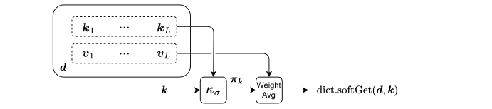
尽管可能的键集合 K\mathcal{K} 可能是无限的,但与某个特定字典 {k1,…,kL}⊂K\{{\bm{k}}_{1},\dots,{\bm{k}}_{L}\}\subset\mathcal{K} 相关联的键集合 d=((k1,v1),…,(kL,vL)){\bm{d}}=(({\bm{k}}_{1},{\bm{v}}_{1}),\dots,({\bm{k}}_{L},{\bm{v}}_{L})) 却是有限的。因此,对某个特定的键 k{\bm{k}},我们可以关联一个定义在 πk=(πk,1,…,πk,L)∈△L{\bm{\pi}}_{\bm{k}}=(\pi_{{\bm{k}},1},\dots,\pi_{{\bm{k}},L})\in\triangle^{L} 的键 (k1,…,kL)({\bm{k}}_{1},\dots,{\bm{k}}_{L}) 上的离散概率分布 d{\bm{d}},其定义为While the set of possible keys K\mathcal{K} is potentially infinite, the set of keys {k1,…,kL}⊂K\{{\bm{k}}_{1},\dots,{\bm{k}}_{L}\}\subset\mathcal{K} associated with a particular dictionary d=((k1,v1),…,(kL,vL)){\bm{d}}=(({\bm{k}}_{1},{\bm{v}}_{1}),\dots,({\bm{k}}_{L},{\bm{v}}_{L})) is finite. To a particular key k{\bm{k}}, we can therefore associate a discrete probability distribution πk=(πk,1,…,πk,L)∈△L{\bm{\pi}}_{\bm{k}}=(\pi_{{\bm{k}},1},\dots,\pi_{{\bm{k}},L})\in\triangle^{L} over the keys (k1,…,kL)({\bm{k}}_{1},\dots,{\bm{k}}_{L}) of d{\bm{d}}, defined by

πk,i:=κσ(k−ki)∑j=1Lκσ(k−kj)∀i∈[L].\pi_{{\bm{k}},i}\coloneqq\frac{\kappa_{\sigma}({\bm{k}}-{\bm{k}}_{i})}{\sum_{j=1}^{L}\kappa_{\sigma}({\bm{k}}-{\bm{k}}_{j})}\quad\forall i\in[L].

该分布刻画了输入键 k{\bm{k}} 与字典 d{\bm{d}} 的键 (k1,…,kL)({\bm{k}}_{1},\dots,{\bm{k}}_{L}) 之间的亲和度。如图 6.3 所示,我们得到This distribution captures the affinity between the input key k{\bm{k}} and the keys (k1,…,kL)({\bm{k}}_{1},\dots,{\bm{k}}_{L}) of dictionary d{\bm{d}}. As illustrated in Fig. 6.3, we obtain

dict.softGet(d,k)\displaystyle\mathrm{dict.softGet}({\bm{d}},{\bm{k}}) =Ei∼Categorical(πk)[vi]\displaystyle=\mathbb{E}_{i\sim\mathrm{Categorical}({\bm{\pi}}_{\bm{k}})}[{\bm{v}}_{i}]
=∑i=1Lπk,ivi.\displaystyle=\sum_{i=1}^{L}\pi_{{\bm{k}},i}{\bm{v}}_{i}.

在极限 σ→0\sigma\to 0 下,我们恢复In the limit σ→0\sigma\to 0, we recover

dict.get(d,k)=∑i=1Leq(k,ki)vi∑i=1Leq(k,ki).\mathrm{dict.get}({\bm{d}},{\bm{k}})=\frac{\sum_{i=1}^{L}\mathrm{eq}({\bm{k}},{\bm{k}}_{i}){\bm{v}}_{i}}{\sum_{i=1}^{L}\mathrm{eq}({\bm{k}},{\bm{k}}_{i})}.
图 6.3:dict.softGet\mathrm{dict.softGet} 函数的计算图。我们可以用核 κσ\kappa_{\sigma} 构造一个离散概率分布 πk=(πk,1,…,πk,L)∈△L{\bm{\pi}}_{\bm{k}}=(\pi_{{\bm{k}},1},\dots,\pi_{{\bm{k}},L})\in\triangle^{L},用以刻画字典键 (k1,…,kL)({\bm{k}}_{1},\dots,{\bm{k}}_{L}) 与输入键 k{\bm{k}} 之间的亲和度。由此,dict.softGet\mathrm{dict.softGet} 函数便可视为以概率值 (πk,1,…,πk,L)(\pi_{{\bm{k}},1},\dots,\pi_{{\bm{k}},L}) 为权重、对取值 (v1,…,vL)({\bm{v}}_{1},\dots,{\bm{v}}_{L}) 所作的凸组合(加权平均)。Figure 6.3: Computation graph of the dict.softGet\mathrm{dict.softGet} function. We can use a kernel κσ\kappa_{\sigma} to produce a discrete probability distribution πk=(πk,1,…,πk,L)∈△L{\bm{\pi}}_{\bm{k}}=(\pi_{{\bm{k}},1},\dots,\pi_{{\bm{k}},L})\in\triangle^{L}, that captures the affinity between the dictionary keys (k1,…,kL)({\bm{k}}_{1},\dots,{\bm{k}}_{L}) and the input key k{\bm{k}}. The dict.softGet\mathrm{dict.softGet} function can then merely be seen as a convex combination (weighted average) of values (v1,…,vL)({\bm{v}}_{1},\dots,{\bm{v}}_{L}) using the probability values (πk,1,…,πk,L)(\pi_{{\bm{k}},1},\dots,\pi_{{\bm{k}},L}) as weights.

dict.get\mathrm{dict.get} 函数使用的是从键 k∈{k1,…,kL}{\bm{k}}\in\{{\bm{k}}_{1},\dots,{\bm{k}}_{L}\} 到整数索引 [L][L] 的映射,而 dict.softGet\mathrm{dict.softGet} 函数使用的则是从键 k∈{k1,…,kL}{\bm{k}}\in\{{\bm{k}}_{1},\dots,{\bm{k}}_{L}\} 到分布 πk∈△L{\bm{\pi}}_{{\bm{k}}}\in\triangle^{L} 的映射。这一视角使我们能够复用 6.1 节中为列表建立的软函数。例如,要软地替换与键 k{\bm{k}} 相关联的取值,我们可以执行以下运算:While the dict.get\mathrm{dict.get} function is using a mapping from keys k∈{k1,…,kL}{\bm{k}}\in\{{\bm{k}}_{1},\dots,{\bm{k}}_{L}\} to integer indices [L][L], the dict.softGet\mathrm{dict.softGet} function is using a mapping from keys k∈{k1,…,kL}{\bm{k}}\in\{{\bm{k}}_{1},\dots,{\bm{k}}_{L}\} to distributions πk∈△L{\bm{\pi}}_{{\bm{k}}}\in\triangle^{L}. This perspective allows us to reuse the soft functions we developed for lists in Section 6.1. For example, we can softly replace the value associated with key k{\bm{k}} by performing

list.softSet(d,πk,(k,v)).\mathrm{list.softSet}({\bm{d}},{\bm{\pi}}_{\bm{k}},({\bm{k}},{\bm{v}})).

与 dict.set\mathrm{dict.set} 不同,该函数关于分布 πk{\bm{\pi}}_{\bm{k}} 是可微的。Unlike dict.set\mathrm{dict.set}, the function is differentiable w.r.t. the distribution πk{\bm{\pi}}_{\bm{k}}.

6.2.4 与 Transformer 中注意力的联系Link with attention in Transformers

当 κσ\kappa_{\sigma} 为高斯核时,若假定键已被归一化为具有单位范数(实际实现中往往如此 [177, 54]),则可得In the case when κσ\kappa_{\sigma} is the Gaussian kernel, assuming that the keys are normalized to have unit norm (which is often the case in practical implementations [177, 54]), we obtain

κσ(k−ki)\displaystyle\kappa_{\sigma}({\bm{k}}-{\bm{k}}_{i}) =exp⁡(−∥k−ki∥22/(2σ2))\displaystyle=\exp(-\|{\bm{k}}-{\bm{k}}_{i}\|^{2}_{2}/(2\sigma^{2}))
=exp⁡(−(∥k∥22+∥ki∥22)/(2σ2))exp⁡(⟨k,ki⟩/σ2)\displaystyle=\exp(-(\|{\bm{k}}\|^{2}_{2}+\|{\bm{k}}_{i}\|^{2}_{2})/(2\sigma^{2}))\exp(\langle{\bm{k}},{\bm{k}}_{i}\rangle/\sigma^{2})
=exp⁡(−1/σ2)exp⁡(⟨k,ki⟩/σ2)\displaystyle=\exp(-1/\sigma^{2})\exp(\langle{\bm{k}},{\bm{k}}_{i}\rangle/\sigma^{2})

于是so that

πk,i\displaystyle\pi_{{\bm{k}},i} =κσ(k−ki)∑j=1Lκσ(k−kj)\displaystyle=\frac{\kappa_{\sigma}({\bm{k}}-{\bm{k}}_{i})}{\sum_{j=1}^{L}\kappa_{\sigma}({\bm{k}}-{\bm{k}}_{j})}
=exp⁡(⟨k,ki⟩/σ2)∑j=1Lexp⁡(⟨k,kj⟩/σ2).\displaystyle=\frac{\exp(\langle{\bm{k}},{\bm{k}}_{i}\rangle/\sigma^{2})}{\sum_{j=1}^{L}\exp(\langle{\bm{k}},{\bm{k}}_{j}\rangle/\sigma^{2})}.

我们认出了 softargmax 算子。因此,给定字典 d=((k1,v1),…,(kL,vL)){\bm{d}}=(({\bm{k}}_{1},{\bm{v}}_{1}),\dots,({\bm{k}}_{L},{\bm{v}}_{L})),便可恢复出 Transformer [199] 中的注意力:We recognize the softargmax operator. Given a dictionary
d=((k1,v1),…,(kL,vL)){\bm{d}}=(({\bm{k}}_{1},{\bm{v}}_{1}),\dots,({\bm{k}}_{L},{\bm{v}}_{L})), we thus recover attention from Transformers [199] as

dict.softGet(d,k)\displaystyle\mathrm{dict.softGet}({\bm{d}},{\bm{k}}) =∑i=1Lπk,ivi\displaystyle=\sum_{i=1}^{L}\pi_{{\bm{k}},i}{\bm{v}}_{i}
=∑i=1Lexp⁡(⟨k,ki⟩/σ2)vi∑j=1Lexp⁡(⟨k,kj⟩/σ2).\displaystyle=\sum_{i=1}^{L}\frac{\exp(\langle{\bm{k}},{\bm{k}}_{i}\rangle/\sigma^{2}){\bm{v}}_{i}}{\sum_{j=1}^{L}\exp(\langle{\bm{k}},{\bm{k}}_{j}\rangle/\sigma^{2})}.

可见,Transformer 可以解释为依赖一种可微的字典机制。除 Transformer 之外,基于内容的记忆寻址也被用于神经图灵机 [82]。Transformers can therefore be interpreted as relying on a differentiable dictionary mechanism. Besides Transformers, content-based memory addressing is also used in neural Turing machines [82].

6.3 小结6.3 Summary

  • •

    列表上的运算关于列表连续且可微,但关于整数索引则不然。类似地,字典上的运算关于字典连续且可微,但关于输入键则不然。Operations on lists are continuous and differentiable w.r.t. the list, but not w.r.t. the integer index. Similarly, operations on dictionaries are continuous and differentiable w.r.t. the dictionary, but not w.r.t. the input key.

  • •

    与我们在条件语句中处理谓词的方式类似,我们可以用索引上的概率分布(相应地,键上的概率分布)替换整数索引(相应地,键)。Similarly to the way we handled the predicate in conditionals, we can replace the integer index (respectively the key) with a probability distribution over the indices (respectively the keys).

  • •

    由此,我们便得到了列表运算的概率松弛。特别地,list.get\mathrm{list.get} 的松弛相当于执行一次卷积,而 dict.get\mathrm{dict.get} 的松弛则相当于用核回归计算一个条件期望。This allows us to obtain a probabilistic relaxation of operations on lists. In particular, the relaxation for list.get\mathrm{list.get} amounts to performing a convolution. The relaxation for dict.get\mathrm{dict.get} amounts to computing a conditional expectation using kernel regression.

  • •

    当使用键被归一化为单位范数的高斯核时,我们便恢复出 Transformer 的 softargmax 注意力。When using a Gaussian kernel with keys normalized to unit norm, we recover softargmax attention from Transformers.