第 2 章 微分Chapter 2 Differentiation
在本章中,我们回顾关键的微分概念。特别地,我们强调线性映射所起的基础性作用。In this chapter, we review key differentiation concepts. In particular, we emphasize the fundamental role played by linear maps.
2.1 一元函数2.1 Univariate functions
2.1.1 导数Derivatives
为了研究函数,我们需要捕捉函数在点附近的无穷小变化,这由极限的概念来定义。To study functions, we need to capture their infinitesimal variations around points as defined by the notion of limit.
定义 2.1.1(极限)。Definition 2.1.1 (Limit).
我们也可以将 写作 。极限在加法与乘法下保持不变。即,若 且 ,则对任意 与 ,记 ,根据极限的定义,我们有 与 。极限在加法与数乘下保持不变,这通常被称为极限的线性性,后续许多定义都继承了这一性质。We can also write as . Limits are preserved under additions and multiplications. Namely, if and , then denoting for any and , we have by definition of the limit, and . The preservation of the limit under addition and multiplication by a scalar is generally referred to as the linearity of the limit, a property that many definitions in the sequel inherit.
借助极限的概念,我们已经可以刻画一类“性态良好”的函数:在任何点处的极限都等于该点处函数值的函数。满足这一性质的函数称为连续函数。With the notion of limit, we can already delineate a class of “well-behaved” functions: functions whose limit at any point equals the value of the function at that point. Functions satisfying this property are called continuous.
定义 2.1.2(连续函数)。Definition 2.1.2 (Continuous function).
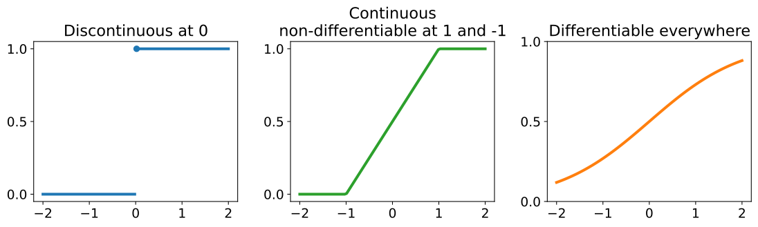
尽管连续性这一概念看似是一个温和的假设,但机器学习中常用的若干函数,例如 Heaviside 阶跃函数(见图 2.2 左图),并不连续,需要特殊处理。Although the notion of continuity appears to be a benign assumption, several functions commonly used in machine learning, such as the Heaviside step function (displayed in the left panel of Fig. 2.2), are not continuous and require special treatment.
注 2.1.3(小 记号)。Remark 2.1.3 (Little notation).
现在我们解释导数。考虑一个函数 。如图 2.1 所示,该函数在区间 上的值可以用其取值 与 之间的割线来近似,这是一条斜率为 的线性函数。在 附近的无穷小变化 的极限下,割线收敛到 在 处的切线,由此得到的斜率定义了 在 处的导数。下面的定义将这一直观形式化。We now explain derivatives. Consider a function . As illustrated in Fig. 2.1, its value on an interval can be approximated by the secant between its values and , a linear function with slope . In the limit of an infinitesimal variation around , the secant converges to the tangent of at and the resulting slope defines the derivative of at . The definition below formalizes this intuition.
定义 2.1.4(导数)。Definition 2.1.4 (Derivative).
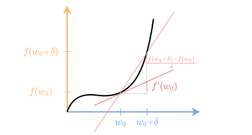
若 在给定的 处可微,则它在该点 处必然连续,如下面的命题所示。连续函数在给定点 处不可微,通常表现为一个折角,如图 2.2 所示。If is differentiable at a given , then it is necessarily continuous at as shown in the following proposition. Non-differentiability of a continuous function at a given point is generally illustrated by a kink, as shown in Fig. 2.2.
命题 2.1.5(可微蕴含连续)。Proposition 2.1.5 (Differentiability implies continuity).
证明 2.1.6。Proof 2.1.6.
用小 记号表示时, 在 处可微,如果存在 ,使得In little notation, is differentiable at if there exists , such that
由于当 时 ,故 在 处连续。Since as , is continuous at .
导数 是 在 处切线的斜率,因而它除了能够构造 在 邻域内的线性近似之外,还能揭示 在 附近的单调性。若 为正,则函数在 附近递增;反之,若 为负,则函数递减。这类信息可用于设计梯度下降等迭代算法:该类算法通过计算形如 (其中 )的迭代值,沿着 在 附近的下降方向不断移动,以最小化 。In addition to enabling the construction of a linear approximation of in a neighborhood of , since it is the slope of the tangent of at , the derivative informs us about the monotonicity of around . If is positive, the function is increasing around . Conversely, if is negative, the function is decreasing. Such information can be used to develop iterative algorithms such as gradient descent, which seeks to minimize by computing iterates of the form for , thereby moving along descent directions of around .
对于若干初等函数,例如 、、、 或 ,其导数均可直接通过应用式 2.1 中导数的定义求得,下面我们对此加以说明。For several elementary functions such as , , , or , their derivatives can be obtained directly by applying the definition of the derivative in Eq. 2.1 as we now illustrate.
例 2.1.7(幂函数的导数)。Example 2.1.7 (Derivative of power function).
注 2.1.8(定义在 的子集 上的函数)。Remark 2.1.8 (Functions on a subset of ).
2.1.2 求导法则Calculus rules
给定 以及两个函数 与 ,只要 与 在 处的可微性满足适当条件,便可根据导数的定义容易地推出对 与 所做初等运算(如求和、求积或复合)的导数。例如,若 与 的导数在 处存在,则其加权和或乘积的导数存在,并满足以下法则For a given and two functions and , the derivative of elementary operations on and such as their sums, products or compositions can easily be derived from the definition of the derivative, under appropriate conditions on the differentiability of and at . For example, if the derivatives of and exist at , then the derivatives of their weighted sum or product exist, and satisfy the rules
| (线性性)(Linearity) | ||
| (乘积法则)(Product rule) |
其中 。线性性可直接由极限的线性性验证。至于乘积法则,采用小 记号,当 时,我们有where . The linearity can be verified directly from the linearity of the limits. For the product rule, in little notation, we have, as ,
由此得证。hence the result.
若 在 处的导数与 在 处的导数均存在,则复合函数 在 处的导数存在,且由下式给出If the derivatives of at and of at exist, then the derivative of the composition at exists and is given by
| (链式法则)(Chain rule) |
我们将在命题 2.2.11 中对这一结果给出更一般的证明。正如后文所示,线性性与乘积法则可视为链式法则的推论,因此链式法则构成了微分学的基石。We prove this result more generally in Proposition 2.2.11. As seen in the sequel, the linearity and the product rule can be seen as byproducts of the chain rule, making the chain rule the cornerstone of differentiation.
考虑一个可由初等函数的和、积或复合表示的函数,例如 。将 分解为初等运算与初等函数,再应用上述法则,即可计算其导数。Consider a function that can be expressed using sums, products or compositions of elementary functions, such as . Its derivative can be computed by applying the aforementioned rules on the decomposition of into elementary operations and functions.
例 2.1.9(应用求导法则)。Example 2.1.9 (Applying rules of differentiation).
这一过程完全是机械性的,因而适合交由自动化流程完成,这正是第 8 章所介绍的自动微分的主要思想。Such a process is purely mechanical and lends itself to an automated procedure, which is the main idea of automatic differentiation presented in Chapter 8.
2.1.3 莱布尼茨记号Leibniz’s notation
导数的概念最早由牛顿与莱布尼茨于 18 世纪各自独立提出 [9]。后者将导数视为无穷小变化量之商。也就是说,记 为通过 依赖于 的变量,莱布尼茨便将 的导数视为如下商The notion of derivative was first introduced independently by Newton and Leibniz in the 18th century [9]. The latter considered derivatives as the quotient of infinitesimal variations. Namely, denoting a variable depending on through , Leibniz considered the derivative of as the quotient
其中 与 分别表示 与 的无穷小变化量,符号 则表示在给定点 处对导数求值。这一记号简化了莱布尼茨最早发现的链式法则 [170] 的表述,因为对于 与 ,我们有where and denote infinitesimal variations of and respectively and the symbol denotes the evaluation of the derivative at a given point . This notation simplifies the statement of the chain rule first discovered by Leibniz [170] as we have for and
这暗示在考虑复合时导数会相乘。求值时,莱布尼茨记号下的链式法则可还原出上文给出的公式:This hints that derivatives are multiplied when considering compositions. At evaluation, the chain rule in Leibniz notation recovers the formula presented above as
莱布尼茨记号能将链式法则表达为商之乘积,这一能力使其在数个世纪以来广受欢迎,尤其是在力学领域 [9]。莱布尼茨记号背后的原理,即“无穷小变化量”这一概念,因其潜在的逻辑问题而受到后来数学家的质疑 [9]。由欧拉首次引入、后经拉格朗日进一步推广的记号 [40] 随之在众多数学教材中占据主流。无穷小变化量的概念已借助超实数集得到严格定义。超实数集将每个数视为非无穷小部分与无穷小部分之和,从而扩展了实数集 [94]。无穷小变化量的形式化还通过对偶数这一概念,进一步支撑了自动微分算法的发展。The ability of Leibniz’s notation to capture the chain rule as a mere product of quotients made it popular throughout the centuries, especially in mechanics [9]. The rationale behind Leibniz’s notation, the concept of “infinitesimal variations”, was questioned by later mathematicians for its potential logical issues [9]. The notation first introduced by Euler and further popularized by Lagrange [40] has then taken over in numerous mathematical textbooks. The concept of infinitesimal variations has been rigorously defined by using the set of hyperreal numbers. They extend the set of real numbers by considering each number as a sum of a non-infinitesimal part and an infinitesimal part [94]. The formalism of infinitesimal variations further underlies the development of automatic differentiation algorithms through the concept of dual numbers.
2.2 多元函数2.2 Multivariate functions
2.2.1 方向导数Directional derivatives
现在我们考虑一个输入为多维的 函数,其输入为 。机器学习中最重要的例子,是这样一个函数:它将神经网络的参数 映射为 中的损失值。 的变化需要沿特定方向定义,例如 在 附近沿方向 发生大小为 的变化 。这一考虑自然引出了方向导数的定义。Let us now consider a function with multi-dimensional input . The most important example in machine learning is a function which, to the parameters of a neural network, associates a loss value in . Variations of need to be defined along specific directions, such as the variation of around in the direction by an amount . This consideration naturally leads to the definition of the directional derivative.
定义 2.2.1(方向导数)。Definition 2.2.1 (Directional derivative).
我们采用记号 ,以强调对给定的输入 ,可将 视为一个函数。这对于定义 在 处的可微性(定义 2.2.3),以及后文定义线性映射(2.3 节),都是必不可少的。We use the notation to emphasize that, for a given input , we can see as a function. This is essential to define the differentiability of (Definition 2.2.3) at and to later define linear maps (Section 2.3).
方向导数的一个例子是:求函数 在 处沿任一标准方向的导数One example of directional derivative consists in computing the derivative of a function at in any of the canonical directions
据此便可定义偏导数的概念,对 记作This allows us to define the notion of partial derivatives, denoted for
用莱布尼茨记号,这也可写作 或 。由于只沿函数的第 个坐标移动,偏导数相当于在其余坐标均固定于 的情形下,对 附近的函数 求导。This is also denoted in Leibniz’s notation as or . By moving along only the th coordinate of the function, the partial derivative is akin to differentiating the function around , letting all other coordinates fixed at their values .
2.2.2 梯度Gradients
下面引入梯度向量,它汇集了各个偏导数。在此之前,先回顾线性映射与线性泛函的定义。We now introduce the gradient vector, which gathers the partial derivatives. We first recall the definitions of linear map and linear form.
定义 2.2.2(线性映射、线性泛函)。Definition 2.2.2 (Linear map, linear form).
线性性在函数的可微性中起着关键作用。Linearity plays a crucial role in the differentiability of a function.
定义 2.2.3(可微性,单输出情形)。Definition 2.2.3 (Differentiability, single-output case).
现在可以引入梯度了。We can now introduce the gradient.
定义 2.2.4(梯度)。Definition 2.2.4 (Gradient).
此处 表示内积,其定义见 2.3.2 节关于欧几里得空间的讨论。Here, denotes the inner product. We provide its definition in Euclidean spaces in Section 2.3.2.
在上述定义中,梯度之所以能用来计算方向导数,不过是 关于 的线性性的一个推论。然而在后文所介绍的更为抽象的情形中,梯度正是通过这一性质直接定义的。In the definition above, the fact that the gradient can be used to compute the directional derivative is a mere consequence of the linearity of w.r.t. . However, in more abstract cases presented in later sections, the gradient is defined directly through this property.
作为一个简单的例子,任何形如 的线性函数都是可微的,因为对任意 都有 ,特别是当 时也成立。此外,其梯度自然由 给出。As a simple example, any linear function of the form is differentiable as we have for any and in particular for . Moreover, its gradient is naturally given by .
更一般地,若要证明一个函数可微并求出其梯度,一种方法是在 附近对 作近似。如果我们能找到一个向量 ,使得More generally, to show that a function is differentiable and find its gradient, one approach is to approximate around . If we can find a vector such that
那么 在 处可微,因为 是线性的。此外,此时 正是 在 处的梯度。then is differentiable at , since is linear. Moreover, is then the gradient of at .
注 2.2.5(Gateaux 可微性与 Fréchet 可微性)。Remark 2.2.5 (Gateaux and Fréchet differentiability).
下一个例子说明如何计算 logistic 损失的梯度,并验证其可微性。The next example illustrates how to compute the gradient of the logistic loss and validates its differentiability.
例 2.2.6(logistic 损失的梯度)。Example 2.2.6 (Gradient of logistic loss).
梯度的线性性Linearity of gradients
多输入函数的可微性概念,自然地继承自单输入函数导数的线性性。对任意 以及任意在 处可微的多输入函数 ,函数 在 处可微,且其梯度为The notion of differentiability for multi-input functions naturally inherits from the linearity of derivatives for single-input functions. For any and any multi-input functions differentiable at , the function is differentiable at and its gradient is
梯度为何有用?Why is the gradient useful?
当 可微时,若满足……则称 是 在 处的上升方向:When is differentiable, we say that is an ascent direction of from if
反之,若满足下式,则称 是 自 出发的一个下降方向:Conversely, we say that is a descent direction of from if
利用这一定义可知,梯度给出了从 出发的 的最陡上升方向。为说明其原因,我们注意到Using this definition, the gradient leads to the steepest ascent direction of from . To see why, we note that
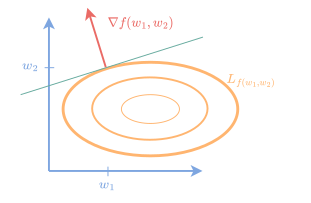
这里我们假设了 。梯度 垂直于该函数的水平集(即满足 的同一取值的点 所构成的集合),并指向 取值更大的方向,如图 2.4 所示。反之,负梯度 则指向 取值更小的方向。正是这一观察推动了梯度下降等优化算法的产生。这类算法对 反复执行更新 ,从而沿最陡下降方向在 附近逐步移动,以寻找 的极小值点;该方向相差一个乘性因子即由 给出。更多细节参见定义 17.1.1。where we assumed . The gradient is orthogonal to the level set of the function (the set of points sharing the same value ) and points towards higher values of , as illustrated in Fig. 2.4. Conversely, the negative gradient points towards lower values of . This observation motivates the development of optimization algorithms such as gradient descent. It is based on iteratively performing the update , for . It therefore seeks for a minimizer of by moving along the steepest descent direction around given, up to a multiplicative factor, by . See also Definition 17.1.1 for more details.
2.2.3 雅可比矩阵Jacobians
下面考虑由 定义的多输出函数 ,其中 。机器学习中的典型例子是神经网络。方向导数的概念可推广到这类函数:将其定义为各坐标方向导数所构成的向量,即Let us now consider a multi-output function defined by , where . A typical example in machine learning is a neural network. The notion of directional derivative can be extended to such function by defining it as the vector composed of the coordinate-wise directional derivatives:
式中极限(若存在)按坐标逐一施加。因此, 沿方向 的方向导数,就是汇集各 方向导数的向量,即 。特别地,可将 在 处的偏导数定义为如下向量where the limits (provided that they exist) are applied coordinate-wise. The directional derivative of in the direction is therefore the vector that gathers the directional derivative of each , i.e., . In particular, we can define the partial derivatives of at as the vectors
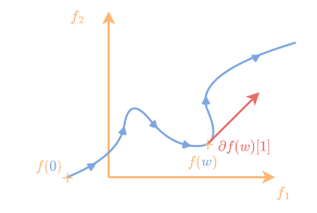
与通常的导数定义一样,方向导数可给出函数在当前输入附近的线性近似,如图 2.4 中参数曲线 所示。As for the usual definition of the derivative, the directional derivative can provide a linear approximation of a function around a current input, as illustrated in Fig. 2.4 for a parametric curve .
与单输出情形相同,可微性不仅要求任意方向上的方向导数都存在,还要求其在所选方向上具有线性性。Just as in the single-output case, differentiability is defined not only as the existence of directional derivatives in any direction but also by the linearity in the chosen direction.
定义 2.2.7(可微性,多输出情形)。Definition 2.2.7 (Differentiability, multi-output case).
各坐标函数的偏导数汇集于雅可比矩阵之中。The partial derivatives of each coordinate’s function are gathered in the Jacobian matrix.
定义 2.2.8(雅可比矩阵)。Definition 2.2.8 (Jacobian).
注意,我们用粗体 表示雅可比矩阵,即将其视为矩阵。雅可比矩阵自然地推广了前文所述的导数与梯度概念。与单输入情形一样,要证明一个函数可微,一种方法是考虑 在 附近的近似。若能找到一个线性映射 使得Notice that we use bold to indicate the Jacobian, seen as a matrix. The Jacobian matrix naturally generalizes the concepts of derivatives and gradients presented earlier. As for the single input case, to show that a function is differentiable, one approach is to approximate around . If we find a linear map such that
则 在 处可微;此外,若 由矩阵 表示,且满足 ,则 。then is differentiable at . Moreover, if is represented by matrix such that then .
举一个简单的例子:任意线性函数 (其中 )都是可微的,因为它的各个按坐标分量都是单输出线性函数,且 在任意 处的雅可比矩阵由 给出。As a simple example, any linear function for is differentiable, since all its coordinate-wise components are single-output linear functions, and the Jacobian of at any is given by .
注 2.2.9(雅可比矩阵的特殊情形)。Remark 2.2.9 (Special cases of the Jacobian).
下例展示了对可微函数 逐元素作用时雅可比矩阵的形式,例如 softplus 激活函数(激活函数的相关回顾见 4.4 节)。此时雅可比矩阵呈现简单的对角矩阵形式。因此,该函数对应的方向导数只需由逐元素乘积给出:无需像定义 2.2.8 所提示的那样进行完整的矩阵—向量乘积。我们将在 2.3 节再次讨论这一点。The next example illustrates the form of the Jacobian matrix for the element-wise application of a differentiable function , such as the softplus activation (see Section 4.4 for a review of activation functions). In this case, the Jacobian takes a simple diagonal matrix form. As a consequence, the directional derivative associated with this function is simply given by an element-wise product: a full matrix-vector product is not needed, as would suggest Definition 2.2.8. We will revisit this point in Section 2.3.
例 2.2.10(softplus 激活函数的雅可比矩阵)。Example 2.2.10 (Jacobian matrix of the softplus activation).
链式法则Chain rule
有了可微性的一般定义以及梯度和雅可比矩阵这些相关对象,我们现在就可以推广此前针对单输入单输出函数引入的链式法则。Equipped with a generic definition of differentiability and the associated objects, gradients and Jacobians, we can now generalize the chain rule, previously introduced for single-input single-output functions.
命题 2.2.11(链式法则)。Proposition 2.2.11 (Chain rule).
证明 2.2.12。Proof 2.2.12.
利用 在 处的可微性以及 在 处的可微性,我们逐步近似 ,We progressively approximate using the differentiability of at and at ,
因此, 在 处可微,其雅可比矩阵为 。Hence, is differentiable at with Jacobian .
命题 2.2.11 堪称一切导数计算的基石。例如,可以借助它重新推导单输入单输出函数导数所对应的线性性与乘积法则。Proposition 2.2.11 can be seen as the cornerstone of any derivative computations. For example, it can be used to rederive the linearity and product rules associated to the derivatives of single-input single-output functions.
当 为标量值时,结合注 2.2.9,便可得到 的一个简洁表达式。When is scalar-valued, combined with Remark 2.2.9, we obtain a simple expression for .
命题 2.2.13(链式法则,标量值情形)。Proposition 2.2.13 (Chain rule, scalar-valued case).
这是机器学习中一个非常有用的恒等式,因为我们经常需要将一个向量值模型函数与一个标量值损失函数复合起来。下面以线性回归为例加以说明。This is a very useful identity in machine learning, as we often need to compose a vector-valued model function and a scalar-valued loss function. We illustrate this with linear regression below.
例 2.2.14(线性回归)。Example 2.2.14 (Linear regression).
2.3 线性映射2.3 Linear maps
雅可比矩阵作为偏导数的一种表示固然有用。然而,可微函数这一概念的核心,以及它在自动微分框架中的实现方式,都在于对两个关键线性映射的获取。这两个映射分别刻画沿输入方向与输出方向的无穷小变化,被称作雅可比—向量乘积(JVP)与向量—雅可比乘积(VJP)。本节将在欧几里得空间的语境下把这些概念形式化。The Jacobian matrix is useful as a representation of the partial derivatives. However, the core idea underlying the definition of differentiable functions, as well as their implementation in an autodiff framework, lies in the access to two key linear maps. These two maps encode infinitesimal variations along input or output directions and are referred to, respectively, as Jacobian-vector product (JVP) and Vector-jacobian product (VJP). This section formalizes these notions, in the context of Euclidean spaces.
2.3.1 线性映射的必要性The need for linear maps
迄今为止,我们讨论的函数 都以向量为输入、以向量为输出。然而在神经网络中,以矩阵乃至张量作为输入或输出的函数同样屡见不鲜。例如,考虑定义在形如 的矩阵上的函数,其中 ,。该函数的输入是矩阵而非向量。当然,我们总可以通过堆叠 的各列,将矩阵 “展平”为向量 。记该操作为 ,其逆操作为 。于是,我们可以等价地把 写作 ,从而沿用先前的框架。然而我们接下来就会看到,这样做效率并不高。So far, we have focused on functions , that take a vector as input and produce a vector as output. However, functions that use matrix or even tensor inputs/outputs are commonplace in neural networks. For example, consider the function of matrices of the form , where and . This function takes a matrix as input, not a vector. Of course, a matrix can always be “flattened” into a vector , by stacking the columns of . We denote this operation by and its inverse by . We can then equivalently write as , so that the previous framework applies. However, we will now see that this would be inefficient.
事实上,由此得到的 在任意 处的雅可比矩阵是一个 大小的矩阵;稍作计算便可看出,其中大部分元素都是零。若要求 在 处沿方向 的方向导数,则需:(i) 将 向量化为 ;(ii) 以 次计算的代价计算矩阵—向量乘积 (此处忽略雅可比矩阵含有大量零元素这一事实);(iii) 将结果重新整形为矩阵。Indeed, the resulting Jacobian of at any consists in a matrix of size , which, after some computations, can be observed to be mostly filled with zeros. Getting the directional derivative of at in a direction would consist in (i) vectorizing into , (ii) computing the matrix-vector product at a cost of computations (ignoring the fact that the Jacobian has many zero entries), (iii) re-shaping the result into a matrix.
另一方面,由于 对其矩阵输入是线性的,可以推知: 在任意 处沿任意方向 的方向导数,恰好就是将该函数自身作用于 的结果。也就是说,有 ;它易于实现,且显然只需 次运算。注意,即便忽略 中的非零元素,代价也依然相同。这里的要点在于:与其使用对应的雅可比矩阵表示,不如把与函数求导相关的运算视为线性映射,如此便能高效利用底层的输入空间或输出空间结构。为此,我们下面回顾在欧几里得空间语境下推广前述定义所必需的主要抽象。On the other hand, since is linear in its matrix input, we can infer that the directional derivative of at any in any direction is simply given by the function itself applied on . Namely, we have , which is simple to implement and clearly only requires operations. Note that the cost would have been the same, had we ignored the non-zero entries of . The point here is that by considering the operations associated to the differentiation of a function as linear maps rather than using the associated representation as a Jacobian matrix, we can efficiently exploit the underlying input or output space structure. To that end, we now recall the main abstractions necessary to extend the previous definitions in the context of Euclidean spaces.
2.3.2 欧几里得空间Euclidean spaces
线性空间又称向量空间,是配备加法规则、且对加法封闭的空间,该加法规则与标量乘法相容(此处我们只限于实数域)。也就是说,在线性空间 中,存在运算 和 ,使得对任意 、 和 ,均有 和 。Linear spaces, a.k.a. vector spaces, are spaces equipped with and closed under an addition rule compatible with multiplication by a scalar (we limit ourselves to the field of reals). Namely, in a linear space , there exist operations and , such that for any , , and , we have and .
欧几里得空间是配备一组基 的线性空间。任意元素 均可分解为 ,其中标量 唯一确定。欧几里得空间的典型例子,是我们已经讨论过的、由所有大小为 的向量构成的集合 。大小为 的矩阵集合 同样自然地构成一个欧几里得空间,它由标准矩阵集 生成:对 ,这些矩阵除第 个元素为 1 之外,其余元素全为零。例如, 可写作 。欧几里得空间天然具有内积的概念。Euclidean spaces are linear spaces equipped with a basis . Any element can be decomposed as for some unique scalars . A canonical example of Euclidean space is the set of all vectors of size that we already covered. The set of matrices of size is also naturally a Euclidean space generated by the set of canonical matrices for filled with zero except at the th entry filled with one. For example, can be written . Euclidean spaces are naturally equipped with a notion of inner product.
定义 2.3.1(内积)。Definition 2.3.1 (Inner product).
由内积诱导的范数定义了 之间的距离 ,从而也给出了收敛性的概念。The norm induced by an inner product defines a distance between , and therefore a notion of convergence.
对于向量,其中 ,内积即通常的内积 。对于矩阵,其中 ,内积即所谓的 Frobenius 内积。它对任意 定义为For vectors, where , the inner product is the usual one For matrices, where , the inner product is the so-called Frobenius inner product. It is defined for any by
其中 是对方阵 定义的迹算子。对于 阶张量——它将矩阵推广到 ——内积同样地对 以如下方式定义:where is the trace operator defined for square matrices . For tensors of order , which generalize matrices to , the inner product is defined similarly for by
其中 是 的第 个元素。where is the th entry of .
2.3.3 线性映射及其伴随Linear maps and their adjoints
定义 2.2.2 中的线性映射概念可直接推广到欧几里得空间。也就是说,从欧几里得空间 到欧几里得空间 的函数 是线性映射,如果对任意 和 ,都有 。当 且 时,总存在矩阵 使得 。因此,我们可以把 看作 作为矩阵的“具体化”。The notion of linear map in Definition 2.2.2 naturally extends to Euclidean spaces. Namely, a function from a Euclidean space onto a Euclidean space is a linear map if for any and , we have . When and , there always exists a matrix such that . Therefore, we can think of as the “materialization” as a matrix of .
例 2.3.2(线性映射)。Example 2.3.2 (Linear map).
我们可以定义线性映射的伴随算子。We can define the adjoint operator of a linear map.
定义 2.3.3(伴随算子)。Definition 2.3.3 (Adjoint operator).
伴随可以看作矩阵转置在线性映射上的对应物。当 时,有 ,这是因为The adjoint can be thought of as the counterpart of the matrix transpose for linear maps. When , we have since
例 2.3.4(伴随线性映射)。Example 2.3.4 (Adjoint linear map).
2.3.4 雅可比矩阵—向量乘积Jacobian-vector products
现在我们用线性映射来定义方向导数,由此引出雅可比—向量乘积(JVP)的概念。这有助于处理定义在张量上的函数,或进一步推广到无穷维空间。下文以 和 表示两个分别配备内积 和 的欧几里得空间。我们首先在一般欧几里得空间中定义可微性。We now define the directional derivative using linear maps, leading to the notion of Jacobian-vector product (JVP). This can be used to facilitate the treatment of functions on tensors or for further extensions to infinite-dimensional spaces. In the following, and denote two Euclidean spaces equipped with inner products and . We start by defining differentiability in general Euclidean spaces.
定义 2.3.5(欧几里得空间中的可微性)。Definition 2.3.5 (Differentiability in Euclidean spaces).
现在我们可以正式定义雅可比矩阵—向量乘积。We can now formally define the Jacobian-vector product.
定义 2.3.6(雅可比矩阵—向量乘积)。Definition 2.3.6 (Jacobian-vector product).
我们再次强调,方向导数 是一个值,而 JVP 是一个函数。严格说来, 可以属于任意欧几里得空间 ,并不一定局限于向量,尽管 JVP 这一缩写会给人这样的暗示。我们之所以采用 JVP 这一名称,是因为它如今已成为标准。We emphasize again that the directional derivative is a value, while the JVP is a function. Strictly speaking, can belong to any Euclidean space and does not need to be limited to a vector, as the JVP acronym would suggest. We adopt the name JVP, as it is now standard.
恢复梯度Recovering the gradient
前面我们看到,对于向量输入、标量输出的可微函数,方向导数等于方向与梯度的内积。对于定义在欧几里得空间上的单输出可微函数,情况亦然,只是此时梯度是输入空间中的元素,内积也相应地取输入空间上的内积。Previously, we saw that for differentiable functions with vector input and scalar output, the directional derivative is equal to the inner product between the direction and the gradient. The same applies when considering differentiable functions from a Euclidean space with single outputs, except that the gradient is now an element of the input space and the inner product is the one associated with the input space.
命题 2.3.7(梯度)。Proposition 2.3.7 (Gradient).
在欧几里得空间中,只需沿 的一组基分解偏导数,即可证明梯度的存在性。这种定义可推广到无穷维空间(例如希尔伯特空间),详见 2.3.9 节。In Euclidean spaces, the existence of the gradient can simply be shown by decomposing the partial derivative along a basis of . Such a definition generalizes to infinite-dimensional (e.g., Hilbert spaces) spaces as discussed in Section 2.3.9.
2.3.5 向量—雅可比矩阵乘积Vector-Jacobian products
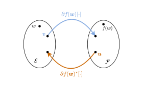
考察函数 。除了考察 沿输入方向 的变化,我们还可以考察 沿输出方向 的变化,即计算标量值函数的梯度 Consider a function . Instead of variations of along an input direction , we may also consider the variations of along an output direction , namely, computing the gradient of the scalar-valued function
等价地,我们也可以计算各坐标函数 在 处的梯度 ,其中 是 中的第 个标准向量。 在 处沿任意输出方向 的无穷小变化由下式给出Equivalently, we may compute the gradients of each coordinate function at , where is the th canonical vector in . The infinitesimal variations of at along any output direction are given by
其中 为雅可比矩阵的转置。利用导数作为极限的定义,对于 ,也可写成where is the Jacobian’s transpose. Using the definition of derivative as a limit, we may also write for
其中 是 中的第 个标准向量。where is the th canonical vector in .
对于一般的欧几里得空间 与 ,转置的对应物是伴随算子,由此引出向量—雅可比乘积的概念。For generic Euclidean spaces and , the counterpart of the transpose is the adjoint operator, leading to the notion of vector-Jacobian product.
命题 2.3.8(向量—雅可比矩阵乘积)。Proposition 2.3.8 (Vector-Jacobian product).
证明 2.3.9。Proof 2.3.9.
命题 2.2.11 给出的链式法则可自然地推广到欧几里得空间(见命题 2.3.10)。由于 是线性的,其方向导数就是其自身。因此, 的方向导数为The chain rule presented in Proposition 2.2.11 naturally generalizes to Euclidean spaces (see Proposition 2.3.10). Since is linear, its directional derivative is itself. Therefore, the directional derivative of is
由于上式对任意 都成立,故依命题 2.3.7, 即为 的梯度。As this is true for any , is the gradient of per Proposition 2.3.7.
图 2.5 展示了 JVP 与 VJP 这两个线性映射。We illustrate the JVP and VJP linear maps in Fig. 2.5.
2.3.6 用线性映射表述的链式法则Chain rule using linear maps
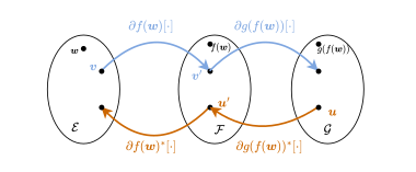
前面用雅可比矩阵表述的链式法则,可以很方便地改写为以 JVP 与 VJP 线性映射实现的形式。The chain rule presented before in terms of Jacobian matrices can readily be formulated to take advantage of the implementations of the JVP and VJP as linear maps.
命题 2.3.10(链式法则,一般情形)。Proposition 2.3.10 (Chain rule, general case).
其证明沿用命题 2.2.11 的证明,图 2.6 给出了相应图示。当最后一个函数取标量值时(这在机器学习中很常见),便得到如下简化结果。The proof follows the one of Proposition 2.2.11. This is illustrated in Fig. 2.6. When the last function is scalar-valued, which is often the case in machine learning, we obtain the following simplified result.
命题 2.3.11(链式法则,标量情形)。Proposition 2.3.11 (Chain rule, scalar case).
2.3.7 多输入函数(扇入)Functions of multiple inputs (fan-in)
函数的输入常常并不只属于一个欧几里得空间,而是属于若干个欧几里得空间的乘积。一个例子是 ,它定义在 上。在这种情况下,将偏导数的概念推广到处理分块输入会较为方便。Oftentimes, the inputs of a function do not belong to only one Euclidean space but to a product of them. An example is , which is defined on . In such a case, it is convenient to generalize the notion of partial derivatives to handle blocks of inputs.
考虑定义在 上的函数 ,其中 。我们将关于第 个输入 沿 的偏导数记为 。借助这一记号,可以分析 JVP 或 VJP 如何沿多个输入进行分解。Consider a function defined on , where . We denote the partial derivative with respect to the th input along as . Equipped with this notation, we can analyze how JVPs or VJPs are decomposed along several inputs.
命题 2.3.12(多输入)。Proposition 2.3.12 (Multiple inputs).
例 2.3.13(矩阵—向量乘积)。Example 2.3.13 (Matrix-vector product).
注 2.3.14(嵌套输入)。Remark 2.3.14 (Nested inputs).
注 2.3.15(隐藏输入)。Remark 2.3.15 (Hiding away inputs).
2.3.8 多输出函数(扇出)Functions with multiple outputs (fan-out)
同样地,处理具有多个输出的函数往往也很方便。Similarly, it is often convenient to deal with functions that have multiple outputs.
命题 2.3.16(多输出)。Proposition 2.3.16 (Multiple outputs).
结合链式法则,我们得到……的雅可比矩阵Combined with the chain rule, we obtain that the Jacobian of
的雅可比矩阵为 ,因此 JVP 为is and therefore the JVP is
2.3.9 推广到非欧几里得线性空间Extensions to non-Euclidean linear spaces
到目前为止,我们关注的都是欧几里得空间,即具有有限基的线性空间。不过,前面讨论的概念可以推广到更一般的空间。So far, we focused on Euclidean spaces, i.e., linear spaces with a finite basis. However, the notions studied earlier can be generalized to more generic spaces.
例如,方向导数(见定义 2.3.5)可以在任何配备范数且关于该范数完备的线性空间中定义,这样的空间称为巴拿赫空间。完备性是一项技术性假设,它要求任何柯西序列都收敛(柯西序列是指随着序列推进,其元素彼此任意接近的序列)。从巴拿赫空间 到巴拿赫空间 的函数 ,若其方向导数沿任意方向都有定义(其中极限是关于 中的范数取的),则称为 Gateaux 可微的。有些作者还要求方向导数必须是线性的,才将函数定义为 Gateaux 可微。For example, directional derivatives (see Definition 2.3.5) can be defined in any linear space equipped with a norm and complete with respect to this norm. Such spaces are called Banach spaces. Completeness is a technical assumption that requires that any Cauchy sequence converges (a Cauchy sequence is a sequence whose elements become arbitrarily close to each other as the sequence progresses). A function defined from a Banach space onto a Banach space is then called Gateaux differentiable if its directional derivative is defined along any direction (where limits are defined w.r.t. the norm in ). Some authors also require the directional derivative to be linear to define a Gateaux differentiable function.
Fréchet 可微性同样可以自然地推广到巴拿赫空间。唯一的区别在于,在一般巴拿赫空间中,满足定义 2.3.5 的线性映射 必须是连续的,即必须存在 ,使得 ,其中 是巴拿赫空间 上的范数。Fréchet differentiability can also naturally be generalized to Banach spaces. The only difference is that, in generic Banach spaces, the linear map satisfying Definition 2.3.5 must be continuous, i.e., there must exist , such that , where is the norm in the Banach space .
梯度与 VJP 的定义则还需要内积的概念。它们可以在希尔伯特空间中定义,即配备了内积、并关于由该内积诱导的范数完备的线性空间(也可以借助对偶空间中的运算,在巴拿赫空间中定义,参见例如 [45])。梯度的存在性由 Riesz 表示定理保证:该定理指出,希尔伯特空间中的任意连续线性泛函,都可以用与某个向量的内积来表示。由于对可微函数 而言,JVP 是一个线性泛函,Riesz 表示定理便保证了梯度的存在,即存在元素 ,使得对任意 都有 。VJP 同样是良定义的,即作为 JVP 关于该希尔伯特空间内积的伴随。The definitions of gradient and VJPs require in addition a notion of inner product. They can be defined in Hilbert spaces, that is, linear spaces equipped with an inner product and complete with respect to the norm induced by the inner product (they could also be defined in a Banach space by considering operations in the dual space, see, e.g. [45]). The existence of the gradient is ensured by Riesz’s representation theorem which states that any continuous linear form in a Hilbert space can be represented by the inner product with a vector. Since for a differentiable function , the JVP is a linear form, Riesz’s representation theorem ensures the existence of the gradient as the element such that for any . The VJP is also well-defined as the adjoint of the JVP w.r.t. the inner product of the Hilbert space.
例如, 上的平方可积函数空间,就是一个配备了内积 的希尔伯特空间。在这里,我们找不到有限个函数,足以表示 上所有可能的函数。因此,这一空间并非单纯的欧几里得空间。尽管如此,我们仍可以考虑这个希尔伯特空间上的函数(称为泛函,以区别于该空间中的元素)。由此定义出的方向导数与梯度,分别称为泛函导数与泛函梯度,参见例如 [72] 及其中的参考文献。As an example, the space of squared integrable functions on is a Hilbert space equipped with the inner product Here, we cannot find a finite number of functions that can express all possible functions on . Therefore, this space is not a mere Euclidean space. Nevertheless, we can consider functions on this Hilbert space (called functionals to distinguish them from the elements of the space). The associated directional derivatives and gradients, can be defined and are called respectively, functional derivative and functional gradient, see, e.g., [72] and references therein.
2.4 二阶微分2.4 Second-order differentiation
2.4.1 二阶导数Second derivatives
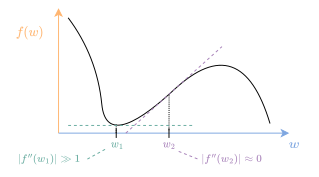
对于单输入单输出的可微函数 ,它在任意一点处的导数本身就是一个函数 。于是,我们可以进一步考虑该导数在任意一点处的导数:二阶导数。For a single-input, single-output differentiable function , its derivative at any point is itself a function . We may then consider the derivative of the derivative at any point: the second derivative.
定义 2.4.1(二阶导数)。Definition 2.4.1 (Second derivative).
若 在给定的 处二阶导数很小,则其导数在 附近几乎为常数。也就是说,函数在 附近的行为近似于一条直线,如图 2.7 所示。因此,二阶导数通常被解释为函数在给定点处的曲率。If has a small second derivative at a given , the derivative around is almost constant. That is, the function behaves like a line around , as illustrated in Fig. 2.7. Hence, the second derivative is usually interpreted as the curvature of the function at a given point.
2.4.2 二阶方向导数Second directional derivatives
对于多输入函数 ,我们已经看到,方向导数刻画了 沿给定方向的无穷小变化。为了分析二阶导数,即函数在给定点 处的曲率,我们可以考虑沿一对方向的变化,其定义如下。For a multi-input function , we saw that the directional derivative encodes infinitesimal variations of along a given direction. To analyze the second derivative, the curvature of the function at a given point , we can consider the variations along a pair of directions, as defined below.
定义 2.4.2(二阶方向导数)。Definition 2.4.2 (Second directional derivative).
特别值得关注的是函数沿标准方向的变化:二阶偏导数,定义为Of particular interest are the variations of a function around the canonical directions: the second partial derivatives, defined as
其中 , 分别为 中的第 个和第 个标准方向。在莱布尼茨记号下,二阶偏导数记为for , the th and th canonical directions in , respectively. In Leibniz notation, the second partial derivatives are denoted
2.4.3 Hessian 矩阵Hessians
对于多输入函数,二次可微性可简单地定义为:任意方向导数 关于 可微。For a multi-input function, twice differentiability is simply defined as the differentiability of any directional derivative w.r.t. .
定义 2.4.3(二次可微性)。Definition 2.4.3 (Twice differentiability).
因此,二阶方向导数是一个双线性型。As a result, the second directional derivative is a bilinear form.
定义 2.4.4(双线性映射、双线性型)。Definition 2.4.4 (Bilinear map, bilinear form).
二阶偏导数汇集于Hessian 矩阵中,而二阶方向导数可由该矩阵计算得到。The second partial derivatives are gathered in the Hessian and the second directional derivatives can be computed from it.
定义 2.4.5(Hessian 矩阵)。Definition 2.4.5 (Hessian).
给定 的梯度,Hessian 矩阵等价于该梯度雅可比矩阵的转置。将记号 稍作推广,用以表示函数雅可比矩阵的转置(这与单输出函数下的定义相符),我们便可将 Hessian 矩阵表示为 ,这也解释了其记号。Given the gradient of , the Hessian is equivalent to the transpose of the Jacobian of the gradient. By slightly generalizing the notation to denote the transpose of the Jacobian of a function (which matches its definition for single-output functions), we have that the Hessian can be expressed as , which justifies its notation.
与函数 的可微性类似, 在 处的二次可微性等价于:二阶偏导数不仅在 的邻域内有定义,而且在该邻域内连续。值得注意的是,要求二次可微,即二阶偏导数连续,就能保证 Hessian 矩阵是对称的 [181]。Similarly as for the differentiability of a function , twice differentiability of at is equivalent to having the second partial derivatives not only defined but also continuous in a neighborhood of . Remarkably, by requiring twice differentiability, i.e., continuous second partial derivatives, the Hessian is guaranteed to be symmetric [181].
命题 2.4.6(Hessian 矩阵的对称性)。Proposition 2.4.6 (Symmetry of the Hessian).
Hessian 矩阵的对称性意味着它也可以写成 ,即 的梯度的雅可比矩阵。The symmetry of the Hessian means that it can alternatively be written as , i.e., the Jacobian of the gradient of .
2.4.4 Hessian 矩阵—向量乘积Hessian-vector products
与雅可比矩阵类似,我们可以利用Hessian 矩阵作为双线性型的形式定义,将其定义推广到欧几里得空间。特别地,我们可以定义Hessian 矩阵—向量乘积这一概念。Similarly to the Jacobian, we can exploit the formal definition of the Hessian as a bilinear form to extend its definition to Euclidean spaces. In particular, we can define the notion of Hessian-vector product.
定义 2.4.7(Hessian 矩阵—向量乘积)。Definition 2.4.7 (Hessian-vector product).
从自动微分的角度看,HVP 可以用四种不同的方式实现,如 9.1 节所述。From an autodiff point of view, the HVP can be implemented in four different ways, as explained in Section 9.1.
2.4.5 二阶雅可比矩阵Second-order Jacobians
前面的定义自然推广到多输出函数 ,其中 ,,且 。二阶方向导数通过汇集各坐标函数的二阶导数来定义。也就是说,对于 ,The previous definitions naturally extend to multi-output functions , where , and . The second directional derivative is defined by gathering the second derivatives of each coordinate’s function. That is, for ,
函数 二次可微,当且仅当其所有坐标都二次可微。此时,二阶方向导数是双线性映射。因此,我们可以按如下方式计算二阶方向导数:The function is twice differentiable if and only if all its coordinates are twice differentiable. The second directional derivative is then a bilinear map. We can then compute second directional derivatives as
当 且 ,从而 时,该双线性映射可以具体化为一个张量When and , so that , the bilinear map can be materialized as a tensor
即 的“二阶雅可比矩阵”。然而,与Hessian 矩阵类似,通常更便于将双线性映射作用于给定向量 和 ,而不是将二阶偏导数具体化为张量。the “second-order Jacobian” of . However, similarly to the Hessian, it is usually more convenient to apply the bilinear map to prescribed vectors and than to materialize the second partial derivatives as a tensor.
2.5 高阶微分2.5 Higher-order differentiation
2.5.1 高阶导数Higher-order derivatives
导数可以推广到任意阶。形式上,对于单输入单输出函数,第 阶导数可以归纳定义如下。Derivatives can be extended to any order. Formally, the th derivative can be defined inductively as follows for a single-input, single-output function.
定义 2.5.1(第 阶导数)。Definition 2.5.1 (th order derivative).
2.5.2 高阶方向导数Higher-order directional derivatives
对于多输入函数 ,我们可以按如下方式自然推广方向导数的概念。For a multi-input function , we can naturally extend the notion of directional derivative as follows.
定义 2.5.2(第 阶方向导数)。Definition 2.5.2 (th order directional derivative).
多输入函数 是 次可微的,如果它 可微,并且它沿任意方向的 阶方向导数都可微。因此,第 阶方向导数是多重线性型。A multi-input function is -times differentiable if it is differentiable and its directional derivative along any direction is differentiable. As a consequence the th directional derivative is a multilinear form.
定义 2.5.3(多重线性映射、多重线性型)。Definition 2.5.3 (Multilinear map, multilinear form).
第 阶方向导数则由下式给出The th order directional derivative is then given by
第 阶偏导数可以具体化为一个 阶张量The th order partial derivatives can be materialized as an th order tensor
2.5.3 高阶雅可比矩阵Higher-order Jacobians
上述所有定义都直接推广到多输出函数 的情形,其中 。此时,第 阶方向导数为All above definitions extend directly to the case of multi-output functions , where . The th directional derivatives are then
函数 称为 次可微的,当它 可微、且沿任意方向的 阶方向导数都可微时。因此,第 阶方向导数是多重线性映射。第 阶方向导数可以分解为偏导数,如下式所示The function is then times differentiable if it is differentiable and its directional derivative along any direction is differentiable. As a consequence, the th directional derivative is a multilinear map. The th directional derivative can be decomposed into partial derivatives as
当 且 时,第 阶偏导数可以通过一个 阶张量具体化When and , the th order partial derivatives can be materialized by an th order tensor
2.5.4 泰勒展开Taylor expansions
借助 Landau 的小 记号,我们已经看到,如果一个函数可微,那么它在 意义下可由一个线性函数逼近,With Landau’s little notation, we have seen that if a function is differentiable, it is approximated by a linear function in ,
将函数展开到其一阶导数的这种做法,称为 在 附近的一阶泰勒展开。Such an expansion of the function up to its first derivative is called the first-order Taylor expansion of around .
若函数 二次可微,则可在 中用二次函数近似它,从而得到 在 附近的二阶泰勒展开,If the function is twice differentiable, we can approximate it by a quadratic in , leading to the second-order Taylor expansion of around ,
与一阶泰勒近似相比,它在 附近自然更为精确,这体现在:对于 ,有 。Compared to the first-order Taylor approximation, it is naturally more accurate around , as reflected by the fact that for .
更一般地,我们可以通过下式构造 次可微函数 在 附近的第 阶泰勒展开More generally, we can build the th order Taylor expansion of a times differentiable function around by
注意,利用变量替换 ,通常可以方便地把 在 附近的第 阶泰勒展开写成Note that, using the change of variable , it is often convenient to write the th Taylor expansion of around as
泰勒展开在第 7 章中对于通过有限差分计算导数将很有用。Taylor expansions will prove useful in Chapter 7 for computing derivatives by finite differences.
2.6 微分几何2.6 Differential geometry
在本章中,我们逐步把导数的概念从实数推广到向量,以及推广到位于线性空间(又称向量空间)中的变量,这些空间既可以是有限维的,也可以是无穷维的。我们还可以通过引入一种局部线性性的概念来进一步推广这些概念。微分几何中的光滑流形对之进行了形式化,其术语常被自动微分文献和软件采用。本节简要概述光滑流形(简称流形)上的导数,完整介绍请参见 [32]。In this chapter, we progressively generalized the notion of derivative from real numbers to vectors and variables living in a linear space (a.k.a. vector space), either finite dimensional or infinite dimensional. We can further generalize these notions by considering a local notion of linearity. This is formalized by smooth manifolds in differential geometry, whose terminology is commonly adopted in the automatic differentiation literature and software. In this section, we give a brief overview of derivatives on smooth manifolds (simply referred to as manifolds), and refer to [32] for a complete introduction.
2.6.1 流形上的可微性Differentiability on manifolds
本质上,流形是一个可以被欧几里得空间局部近似的集合。最常见的例子是像地球这样的球面。从月球上看,地球并不是一个平面,但在人类尺度上局部来看,它可以被视为一个平坦的表面。欧几里得空间也是流形的平凡例子。例 2.6.7 给出了球面作为流形的形式化刻画。目前,我们可以把“流形”视为包含在某个环境欧几里得空间中的某个集合(例如球面);但请注意,流形一般也可以在不包含于欧几里得空间的情况下定义[32,第 8 章]。流形上的可微性直接继承自环境欧几里得空间中的可微性概念。Essentially, a manifold is a set that can be locally approximated by a Euclidean space. The most common example is a sphere like the Earth. Seen from the Moon, the Earth is not a plane, but locally, at a human level, it can be seen as a flat surface. Euclidean spaces are also trivial examples of manifolds. A formal characterization of the sphere as a manifold is presented in Example 2.6.7. For now, we may think of a “manifold” as some set (e.g., the sphere) contained in some ambient Euclidean space; note however that manifolds can be defined generally without being contained in a Euclidean space [32, Chapter 8]. Differentiability in manifolds is simply inherited from the notion of differentiability in the ambient Euclidean space.
定义 2.6.1(受限函数的可微性)。Definition 2.6.1 (Differentiability of restricted functions).
我们的目标是为定义在流形上的函数形式化地给出方向导数与梯度。这一形式化将引出切空间与余切空间的定义,并引出 JVP 与 VJP 算子分别作为前推算子与拉回算子的相应推广。Our objective is to formalize the directional derivatives and gradients for functions defined on manifolds. This formalization leads to the definitions of tangent spaces and cotangent spaces, and the associated generalizations of JVP and VJP operators as pushforward and pullback operators, respectively.
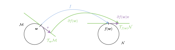
2.6.2 切空间与前推算子Tangent spaces and pushforward operators
为推广函数 的方向导数这一概念,我们希望保留的性质是链式法则。我们不再从 在给定点沿某一方向的变化入手,而是从 沿曲线的变化入手。也就是说,对于像 中的球面 这样的流形,可以考察在时刻 经过 的曲线 ,即 。对于像 这样的单输入函数,为简便起见我们记作 。函数 的方向导数通常须用来定义 在 处的导数,使得 。在球面的情形中,如图 2.8 所示,经过点 的曲线 的导数 总在 处与球面相切。于是,球面在 处的切平面便涵盖了传入我们正在构建的 JVP 的所有可能的相关向量。因此,为定义流形上函数 的方向导数,我们将讨论范围限定在定义于切空间 上的算子;下文中该定义已按我们的需要作了简化。To generalize the notion of directional derivatives of a function , the one property we want to preserve is the chain rule. Rather than starting from the variations of at a given point along a direction, we start with the variations of along curves. Namely, on a manifold like the sphere in , we can look at curves passing through at time , that is, . For single-input functions like , we denote for simplicity . The directional derivative of a function must typically serve to define the derivative of at , such that . In the case of the sphere, as illustrated in Fig. 2.8, the derivative of a curve passing through a point is always tangent to the sphere at . The tangent plane to the sphere at then captures all possible relevant vectors to pass to the JVP we are building. To define the directional derivative of a function on a manifold, we therefore restrict ourselves to an operator defined on the tangent space , whose definition below is simplified for our purposes.
定义 2.6.2(切空间)。Definition 2.6.2 (Tangent space).
就图 2.8 中的球面而言,其切空间是一个平面,也就是一个欧几里得空间。这一性质具有普遍性:切空间都是欧几里得空间,因而我们可以把方向导数定义为线性映射。若 可微,并将流形 映射到流形 ,则 便是 中的一条可微曲线。因此, 是经过 的曲线在 处的导数,且与 在 处相切。于是, 在 处的方向导数可定义为从 在 处的切空间 映入 在 处的切空间 的函数。概而言之,我们考察 与任意曲线 的组合如何将 的导数前推为 的导数,由此构造出方向导数(JVP)。这样得到的 JVP 在微分几何中称为前推算子。In the case of the sphere in Fig. 2.8, the tangent space is a plane, that is, a Euclidean space. This property is generally true: tangent spaces are Euclidean spaces, enabling us to define directional derivatives as linear maps. Now, if is differentiable and goes from a manifold to a manifold , then is a differentiable curve in . Therefore, is the derivative of a curve passing through at and is tangent to at . Hence, the directional derivative of at can be defined as a function from the tangent space of at onto the tangent space of at . Overall, we built the directional derivative (JVP) by considering how a composition of with any curve pushes forward the derivative of into the derivative of . The resulting JVP is called a pushforward operator in differentiable geometry.
定义 2.6.3(前推算子)。Definition 2.6.3 (Pushforward operator).
2.6.3 余切空间与拉回算子Cotangent spaces and pullback operators
为推广 JVP,我们将 与任意在流形上取值的单输入函数 复合。于是,任何这样的 的导数随后从 被前推到 ,这是通过 的作用实现的。为定义 VJP,我们采用对称的方法。我们考虑所有单输出可微函数 ,它们定义在 上,并且具有如下性质: 对某个 成立。然后,我们想要在将 用 预复合时,拉回其导数。因此,VJP 作用的空间是任意 在 处的方向导数构成的空间,这定义了余切空间。To generalize the JVP, we composed with any single-input function giving values on the manifold. The derivative of any such is then pushed forward from to by the action of . To define the VJP, we take a symmetric approach. We consider all single-output differentiable functions defined on with for some . We then want to pull back the derivatives of when precomposing it by . Therefore, the space on which the VJP acts is the space of directional derivatives of any at , defining the cotangent space.
定义 2.6.4(余切空间)。Definition 2.6.4 (Cotangent space).
注意,余切空间的元素是线性映射,而非向量。这一区分之所以重要,是因为在测度论中,拉回算子正是被定义为作用于函数的算子。从线性代数的角度看,余切空间恰是 的对偶空间,即由 到 的线性映射所构成的集合,其中的元素称为线性泛函。由于 是欧几里得空间,其对偶空间 也是欧几里得空间。于是,拉回算子便定义为这样的算子:给定 在 处的方向导数,它便能给出 的方向导数。Note that elements of the cotangent space are linear mappings, not vectors. This distinction is important to define the pullback operator as an operator on functions as done in measure theory. From a linear algebra viewpoint, the cotangent space is exactly the dual space of , that is, the set of linear maps from to , called linear forms. As is a Euclidean space, its dual space is also a Euclidean space. The pullback operator is then defined as the operator that gives access to directional derivatives of given the directional derivative of at .
定义 2.6.5(拉回算子)。Definition 2.6.5 (Pullback operator).
与前推算子作用于向量不同,拉回算子作用于线性泛函。因此, 与 ——即 的伴随算子——在记号上略有差异。为恰当地定义伴随算子 ,我们需要引入内积的概念。由于切空间都是欧几里得空间,我们可以对每个 和 定义内积 ,从而使 成为黎曼流形。有了这些内积,余切空间便可与切空间等同起来,我们也就可以定义梯度了。Contrary to the pushforward operator that acts on vectors, the pullback operator acts on linear forms. Hence, the slight difference in notation between and , the adjoint operator of . To properly define the adjoint operator , we need a notion of inner product. Since tangent spaces are Euclidean spaces, we can define an inner product for each and , making a Riemannian manifold. Equipped with these inner products, the cotangent space can be identified with the tangent space, and we can define gradients.
定义 2.6.6(黎曼流形中的梯度)。Definition 2.6.6 (Gradients in Riemannian manifolds).
因此,与其对方向导数作拉回,不如对梯度作拉回。相应的算子自然就是前推算子的伴随 。具体而言,给定两个黎曼流形 与 ,以及一个可微函数 ,我们有Therefore, rather than pulling back directional derivatives, we can pull back gradients. The corresponding operator is then naturally the adjoint of the pushforward operator. Namely, given two Riemannian manifolds and , and a differentiable function , we have
其中 由 表示。for represented by .
| 函数Function | ||
|---|---|---|
| 前推Push-forward | ||
| 拉回Pullback | ||
| 前推算子的伴随Adjoint of pushforward |
例 2.6.7(球面作为流形)。Example 2.6.7 (The sphere as a manifold).
2.7 广义导数2.7 Generalized derivatives
本书主要关注可微函数,但刻画不可微函数同样重要。这里我们区分两种情形:连续函数与非连续函数。对于前者,存在方向导数、梯度与雅可比矩阵等概念的推广,下文将逐一介绍。对于非连续函数,即便导数几乎处处存在,它们也可能不提供有用信息。例如,控制流(第 5 章)中遇到的分段常值函数几乎处处可微,但导数几乎处处为零。在此类情形下,可以定义替代函数以确保程序的可微性(第四部分)。While we largely focus on differentiable functions in this book, it is important to characterize non-differentiable functions. We distinguish here two cases: continuous functions and non-continuous functions. For the former case, there exist generalizations of the notion of directional derivative, gradient and Jacobian, presented below. For non-continuous functions, even if derivatives exist almost everywhere, they may be uninformative. For example, piecewise-constant functions, encountered in e.g. control flows (Chapter 5), are almost everywhere differentiable but with zero derivatives. In such cases, surrogate functions can be defined to ensure the differentiability of a program (Part IV).
2.7.1 Rademacher 定理Rademacher’s theorem
我们首先回顾(局部)Lipschitz 连续函数的定义。We first recall the definition of (locally) Lipschitz continuous function.
定义 2.7.1((局部)Lipschitz 连续函数)。Definition 2.7.1 ((Locally) Lipschitz continuous function).
Rademacher 定理 [163] 随后保证 几乎处处可微。Rademacher’s theorem [163] then ensures that is differentiable almost everywhere.
命题 2.7.2(Rademacher 定理)。Proposition 2.7.2 (Rademacher’s theorem).
标准证明亦可参见 [139]。See also [139] for a standard proof.
2.7.2 Clarke 导数Clarke derivatives
Rademacher 定理暗示,方向导数、梯度与雅可比矩阵的定义可以推广到局部 Lipschitz 连续函数。这正是 [46] 在其开创性工作中所做的,该工作奠定了非光滑分析的基础。第一个基本构件是广义方向导数的概念。Rademacher’s theorem hints that the definitions of directional derivatives, gradients and Jacobians may be generalized to locally Lipschitz continuous functions. This is what [46] did in his seminal work, which laid the foundation of nonsmooth analysis. The first building block is a notion of generalized directional derivative.
定义 2.7.3(Clarke 广义方向导数)。Definition 2.7.3 (Clarke generalized directional derivative).
与方向导数的通常定义相比,此定义有两点不同:(i) 我们考察的是该点邻域内函数的斜率,而非给定点处的斜率;(ii) 我们取上极限,而非通常的极限。第一点从 Rademacher 定理来看颇为自然:既然函数可微之处的变化能够被恰当刻画,我们便可把这些斜率的极限当作所关注点斜率的候选。第二点更具技术性,却也必不可少:它使我们得以将方向导数刻画为某些线性泛函的上确界 [45];而这些线性泛函反过来又定义了一组广义梯度 [45,第 2 章]。There are two differences with the usual definition of a directional derivative: (i) we consider slopes of the function in a neighborhood of the point rather than at the given point, (ii) we take a limit superior rather than a usual limit. The first point is rather natural in the light of Rademacher’s theorem: we can properly characterize variations on points where the function is differentiable, therefore we may take the limits of these slopes as a candidate slope for the point of interest. The second point is more technical but essential: it allows us to characterize the directional derivative as the supremum of some linear forms [45]. These linear forms in turn define a set of generalized gradients [45, Chapter 2].
定义 2.7.4(Clarke 广义梯度)。Definition 2.7.4 (Clarke generalized gradient).
定义 2.7.3 和定义 2.7.4 适用于非欧几里得空间,例如巴拿赫空间或希尔伯特空间 [45]。在欧几里得空间中,借助 Rademacher 定理,Clarke 广义梯度可以得到更简洁的刻画 [45,定理 8.1]。也就是说,如下文所示,它们可定义为 的梯度在一列收敛于 的序列 上取值的极限的凸组合。Definition 2.7.3 and Definition 2.7.4 can be used in non-Euclidean spaces, such as Banach or Hilbert spaces [45]. In Euclidean spaces, the Clarke generalized gradients can be characterized more simply thanks to Rademacher’s theorem [45, Theorem 8.1]. Namely, as shown below, they can be defined as a convex combination of limits of gradients of evaluated at a sequence in that converges to .
命题 2.7.5(Clarke 广义梯度的刻画)。Proposition 2.7.5 (Characterization of Clarke generalized gradients).
上文中,集合 的凸包——即由 中元素的凸组合构成的集合——记作In the above, the convex hull of a set , the set of convex combinations of elements of , is denoted
两个欧几里得空间之间的函数 的雅可比矩阵也可类似地推广 [45,第 3.3 节]。The Jacobian of a function between two Euclidean spaces can be generalized similarly [45, Section 3.3].
定义 2.7.6(Clarke 广义雅可比矩阵)。Definition 2.7.6 (Clarke generalized Jacobian).
对于连续可微函数 或 ,广义梯度唯一存在,并还原出通常的梯度 [45,命题 3.1,第 78 页]。链式法则也可推广至这些对象 [45]。近来,[30, 29] 通过定义保守梯度,进一步推广了 Clarke 梯度,从而为非光滑函数构造出自动微分方案。For a continuously differentiable function or , there is a unique generalized gradient, recovering the usual gradient [45, Proposition 3.1, page 78]. The chain rule can be generalized to these objects [45]. Recently, [30, 29] further generalized Clarke gradients through the definition of conservative gradients to define automatic differentiation schemes for nonsmooth functions.
2.8 小结2.8 Summary
- •
实值一元函数导数的通常定义,经由在 处沿方向 的方向导数 这一概念,推广到了多元函数 。The usual definition of derivatives of real-valued univariate functions extends to multivariate functions through the notion of directional derivative at in the direction .
- •
为了利用标准基 来表示 ,可微函数的定义要求方向导数关于方向 具有线性性。To take advantage of the representation of using the canonical bases , the definition of differentiable functions requires the linearity of the directional derivative w.r.t. the direction .
- •
这一要求引出了梯度 的概念:它汇集了各偏导数,并进一步确定了在 处的最陡上升方向。This requirement gives rise to the notion of gradient , the vector that gathers the partial derivatives and further defines the steepest ascent direction at .
- •
对于向量输入、向量输出的函数 ,方向导数引出了雅可比矩阵 的定义,该矩阵汇集了所有偏导数(注意我们使用粗体 )。于是,链式法则即为雅可比矩阵的乘积。For vector-input vector-output functions , the directional derivative leads to the definition of Jacobian matrix , the matrix which gathers all partial derivatives (notice that we use bold ). The chain rule is then the product of Jacobian matrices.
- •
这些概念可推广到一般的欧几里得空间,例如矩阵空间或张量空间。对于形如 的函数,其梯度为 。更一般地,对于形如 的函数,雅可比矩阵 可视为一个线性映射(注意此处 未加粗)。在 处的方向导数自然地定义了一个线性映射 ,其中 称为雅可比—向量乘积(JVP),它刻画了在 处沿输入方向 的无穷小变化。These notions can be extended to general Euclidean spaces, such as the spaces of matrices or tensors. For functions of the form , the gradient is . More generally, for functions of the form , the Jacobian can be seen as a linear map (notice the non-bold ). The directional derivative at naturally defines a linear map , where is called the Jacobian vector product (JVP) and captures the infinitesimal variation at along the input direction .
- •
其伴随 定义了另一个线性映射 ,称为向量—雅可比乘积(VJP),它刻画了在 处沿输出方向 的无穷小变化。于是,链式法则即为这些线性映射的组合。Its adjoint defines another linear map called the vector Jacobian product (VJP) and captures the infinitesimal variation at along the output direction . The chain rule is then the composition of these linear maps.
- •
对于将标量值函数 (例如损失函数)与向量值函数 (例如网络函数)进行组合的特殊情形,梯度由 给出。正因如此,能够将伴随作用于梯度——正如我们将看到的,这可以通过反向模式自动微分来实现——在机器学习中才如此普遍。For the particular case when we compose a scalar-valued function (such as a loss function) with a vector-valued function (such as a network function), the gradient is given by . This is why being able to apply the adjoint to a gradient, which as we shall see can be done with reverse-mode autodiff, is so pervasive in machine learning.
- •
JVP 与 VJP 算子的定义还可以在微分几何的语境中进一步推广。在该框架下,JVP 相当于作用于切向量的前推算子,VJP 则相当于作用于余切向量的拉回算子。The definitions of JVP and VJP operators can further be generalized in the context of differentiable geometry. In that framework, the JVP amounts to the pushforward operator that acts on tangent vectors. The VJP amounts to the pullback operator that acts on cotangent vectors.
- •
我们还看到,从 到 的函数 的 Hessian 矩阵记为 。若二阶偏导数连续,则该矩阵是对称的。将其视为线性映射,Hessian 矩阵引出了 Hessian—向量乘积(HVP)的概念;我们看到,它可以归结为 的 JVP 或 VJP。We also saw that the Hessian matrix of a function from to is denoted . It is symmetric if the second partial derivatives are continuous. Seen as linear map, the Hessian leads to the notion of Hessian-vector product (HVP), which we saw can be reduced to the JVP or the VJP of .
- •
本章的主要要点是:计算函数组合的方向导数或梯度,并不需要计算中间雅可比矩阵,而只需计算与这些中间函数相关联的线性映射(JVP 或 VJP)。第 8 章介绍自动微分,其目标正是为计算链、或更一般地为计算图,提供这些映射的高效实现。The main take-away message of this chapter is that computing the directional derivative or the gradient of compositions of functions does not require computing intermediate Jacobians but only to evaluate linear maps (JVPs or VJPs) associated with these intermediate functions. The goal of automatic differentiation, presented in Chapter 8, is precisely to provide an efficient implementation of these maps for computation chains or more generally for computation graphs.