目录通过积分进行平滑

第 14 章 通过积分进行平滑Chapter 14 Smoothing by integration

在本章中,我们回顾基于卷积的平滑技术。In this chapter, we review smoothing techniques based on convolution.

14.1 卷积14.1 Convolution

14.1.1 卷积算子Convolution operators

两个函数 ff 与 gg 之间的卷积会生成另一个函数,记为 f∗gf\ast g。其定义为The convolution between two functions ff and gg produces another function, denoted f∗gf\ast g. It is defined by

(f∗g)(μ):=∫−∞∞f(u)g(μ−u) du,(f\ast g)(\mu)\coloneqq\int_{-\infty}^{\infty}f(u)g(\mu-u)\,du, (14.1)

这里假设积分是良定义的。因此,它是将 ff 与 gg 的乘积,在将 gg 关于 yy 轴作反射并平移之后进行积分所得的结果。这一运算可以视为滑动平均的推广。利用变量替换 u:=μ+zu\coloneqq\mu+z,我们也可以将其写成assuming that the integral is well-defined. It is therefore the integral of the product of ff and gg after gg is reflected about the yy-axis and shifted. It can be seen as a generalization of the moving average. Using the change of variable u:=μ+zu\coloneqq\mu+z, we can also write

(f∗g)(μ)\displaystyle(f\ast g)(\mu) =∫−∞∞f(μ+z)g(−z) dz\displaystyle=\int_{-\infty}^{\infty}f(\mu+z)g(-z)\,dz (14.2)
=∫∞−∞f(μ−v)g(v) (−dv)\displaystyle=\int_{\infty}^{-\infty}f(\mu-v)g(v)\,(-dv)
=∫−∞∞g(v)f(μ−v) dv\displaystyle=\int_{-\infty}^{\infty}g(v)f(\mu-v)\,dv
=(g∗f)(μ).\displaystyle=(g\ast f)(\mu).

因此,卷积算子是可交换的。The convolution operator is therefore commutative.

注 14.1.1(变量替换)。Remark 14.1.1 (Change of variables).
具有信号处理背景的读者或许会觉得,为证明卷积的交换律而作变量替换 u:=μ+zu\coloneqq\mu+z 略显不寻常,因为用 u:=μ−zu\coloneqq\mu-z 能更直接地证明交换律。然而我们在此有意采用 u:=μ+zu\coloneqq\mu+z,因为这样可使我们的记号与第 12.4.1 节的位置—尺度变换 U:=μ+σZU\coloneqq{\bm{\mu}}+\sigma Z 完全一致,从而能够将卷积平滑自然地解释为注入加性噪声。Readers with a background in signal processing might find the change of variables u:=μ+zu\coloneqq\mu+z slightly unconventional for proving the commutativity of the convolution, as u:=μ−zu\coloneqq\mu-z more directly proves commutativity. However, we intentionally use u:=μ+zu\coloneqq\mu+z here, as this perfectly aligns our notation with the location-scale transform U:=μ+σZU\coloneqq{\bm{\mu}}+\sigma Z from Section 12.4.1. It allows us to seamlessly interpret smoothing by convolution as the injection of additive noise.

14.1.2 与核函数的卷积Convolution with a kernel

卷积经常与核函数 κ\kappa 一起使用,以构造 ff 的光滑近似 f∗κf\ast\kappa。最常用的核函数是宽度为 σ\sigma 的高斯核,其定义为The convolution is frequently used together with a kernel κ\kappa to create a smooth approximation f∗κf\ast\kappa of ff. The most frequently used kernel is the Gaussian kernel with width σ\sigma, defined by

κσ(z):=12πσe−12(zσ)2.\kappa_{\sigma}(z)\coloneqq\frac{1}{\sqrt{2\pi}\sigma}e^{-\frac{1}{2}(\frac{z}{\sigma})^{2}}.

这是均值为零、方差为 σ2\sigma^{2} 的正态分布的概率密度函数(PDF)。项 12πσ\frac{1}{\sqrt{2\pi}\sigma} 是归一化常数,它确保该核函数关于 σ\sigma 的求和(积分)为 11。因此,我们说 κσ\kappa_{\sigma} 是归一化核。This is the probability density function (PDF) of the normal distribution with zero mean and variance σ2\sigma^{2}. The term 12πσ\frac{1}{\sqrt{2\pi}\sigma} is a normalization constant, ensuring that the kernel sums to 11 for all σ\sigma. We therefore say that κσ\kappa_{\sigma} is a normalized kernel.

平均视角Averaging perspective

应用式 14.1 中卷积的定义,我们得到Applying the definition of the convolution in Eq. 14.1, we obtain

(f∗κσ)(μ)\displaystyle(f\ast\kappa_{\sigma})(\mu) :=12πσ∫−∞∞f(u)e−12(μ−uσ)2du\displaystyle\coloneqq\frac{1}{\sqrt{2\pi}\sigma}\int_{-\infty}^{\infty}f(u)e^{-\frac{1}{2}(\frac{\mu-u}{\sigma})^{2}}du
=EU∼pμ,σ[f(U)],\displaystyle=\mathbb{E}_{U\sim p_{\mu,\sigma}}[f(U)],

其中where

pμ,σ(u):=κσ(μ−u)=12πσe−12(μ−uσ)2p_{\mu,\sigma}(u)\coloneqq\kappa_{\sigma}(\mu-u)=\frac{1}{\sqrt{2\pi}\sigma}e^{-\frac{1}{2}(\frac{\mu-u}{\sigma})^{2}}

是均值为 μ\mu、方差为 σ2\sigma^{2} 的高斯分布的 PDF。因此,我们可以把 f∗κσf\ast\kappa_{\sigma} 视为 f(u)f(u) 在以 μ\mu 为中心的高斯分布上的期望。这一性质对所有平移不变的核都成立,它们对应于位置—尺度族分布(例如 Laplace 分布)。因此,卷积是对所有点进行平均,其中 μ\mu 附近的点被该分布赋予更大的权重。参数 σ\sigma 控制我们希望给予更远点多大的重要性。我们称这一视角为平均视角,因为我们用 E[f(U)]\mathbb{E}[f(U)] 替换了 f(u)f(u)。is the PDF of the Gaussian distribution with mean μ\mu and variance σ2\sigma^{2}. Therefore, we can see f∗κσf\ast\kappa_{\sigma} as the expectation of f(u)f(u) over a Gaussian centered around μ\mu. This property is true for all translation-invariant kernels, that correspond to a location-scale family distribution (e.g., the Laplace distribution). The convolution therefore performs an averaging with all points, with points nearby μ\mu given more weight by the distribution. The parameter σ\sigma controls the importance we want to give to farther points. We call this viewpoint averaging, as we replace f(u)f(u) by E[f(U)]\mathbb{E}[f(U)].

扰动视角Perturbation perspective

反之,利用式 14.2 中卷积算子的另一种定义(它源于卷积的交换性),我们有Conversely, using the alternative definition of the convolution operator in Eq. 14.2, which stems from the commutativity of the convolution, we have

(f∗κσ)(μ)\displaystyle(f\ast\kappa_{\sigma})(\mu) :=∫−∞∞f(μ+z)e−12(−zσ)2dz\displaystyle\coloneqq\int_{-\infty}^{\infty}f(\mu+z)e^{-\frac{1}{2}(\frac{-z}{\sigma})^{2}}dz
=∫−∞∞f(μ+z)e−12(zσ)2dz\displaystyle=\int_{-\infty}^{\infty}f(\mu+z)e^{-\frac{1}{2}(\frac{z}{\sigma})^{2}}dz
=EZ∼p0,σ[f(μ+Z)],\displaystyle=\mathbb{E}_{Z\sim p_{0,\sigma}}[f(\mu+Z)],

其中,第二行用到了高斯核 p0,σp_{0,\sigma} 的符号不变性,即 p0,σ(−z)=p0,σ(z)p_{0,\sigma}(-z)=p_{0,\sigma}(z)。这一视角表明,用高斯核进行卷积平滑也可以看作是对函数的输入注入高斯噪声或扰动。where, in the second line, we used that the Gaussian kernel p0,σp_{0,\sigma} is sign invariant, i.e., p0,σ(−z)=p0,σ(z)p_{0,\sigma}(-z)=p_{0,\sigma}(z). This viewpoint shows that smoothing by convolution with a Gaussian kernel can also be seen as injecting Gaussian noise or perturbations to the function’s input.

极限情形Limit case

当 σ→0\sigma\to 0 时,核函数 κσ\kappa_{\sigma} 收敛到 Dirac delta 函数,When σ→0\sigma\to 0, the kernel κσ\kappa_{\sigma} converges to a Dirac delta function,

lim⁡σ→0κσ(z)=δ(z).\lim_{\sigma\to 0}\kappa_{\sigma}(z)=\delta(z).

由于 Dirac delta 是卷积代数的乘法单位元(这也称为筛选性质),当 σ→0\sigma\to 0 时,f∗κσf\ast\kappa_{\sigma} 收敛到 ff,即Since the Dirac delta is the multiplicative identity of the convolution algebra (this is also known as the sifting property), when σ→0\sigma\to 0, f∗κσf\ast\kappa_{\sigma} converges to ff, i.e.,

lim⁡σ→0(f∗κσ)(u)=f(u).\lim_{\sigma\to 0}(f\ast\kappa_{\sigma})(u)=f(u).

14.1.3 离散卷积Discrete convolution

很多时候,我们所处理的函数,其卷积并无解析形式。此时,可以在数值网格上采用离散卷积。对于定义在 Z\mathbb{Z} 上的两个函数 ff 与 gg,离散卷积定义为Many times, we work with functions whose convolution does not have an analytical form. In these cases, we can use a discrete convolution on a grid of values. For two functions ff and gg defined over Z\mathbb{Z}, the discrete convolution is defined by

(f∗g)[i]:=∑j=−∞∞f[j]g[i−j].(f\ast g)[i]\coloneqq\sum_{j=-\infty}^{\infty}f[j]g[i-j].

与连续情形相同,离散卷积也是可交换的,即As for its continuous counterpart, the discrete convolution is commutative, namely,

(f∗g)[i]=∑j=−∞∞f[i−j]g[j]=(g∗f)[i].(f\ast g)[i]=\sum_{j=-\infty}^{\infty}f[i-j]g[j]=(g\ast f)[i].

当 gg 在集合 S:={−M,−M+1,…,0,…,M−1,M}S\coloneqq\{-M,-M+1,\dots,0,\dots,M-1,M\} 上具有有限支撑集,即对任意 i∉Si\not\in S 都有 g[i]=0g[i]=0 时,便可将求和限制在有限范围内,即When gg has finite support over the set S:={−M,−M+1,…,0,…,M−1,M}S\coloneqq\{-M,-M+1,\dots,0,\dots,M-1,M\}, meaning that g[i]=0g[i]=0 for all i∉Si\not\in S, a finite summation may be used instead, i.e.,

(f∗g)[i]=∑j=−MMf[i−j]g[j]=(g∗f)[i].(f\ast g)[i]=\sum_{j=-M}^{M}f[i-j]g[j]=(g\ast f)[i].

在实践中,离散信号 f ⁣:Z→Rf\colon\mathbb{Z}\to\mathbb{R} 与连续核函数 κ ⁣:R→R\kappa\colon\mathbb{R}\to\mathbb{R} 之间的卷积,是通过对核函数做离散化来实现的。最简单的做法之一,是在一段区间上取采样点,在这些点上对核函数求值,再将所得的值重新归一化,使采样后的核函数之和为 11。图 14.1 以高斯核为例展示了这一做法。由于高斯核按指数速度衰减,我们可以围绕 00 选取一个较窄的区间。关于高斯核其他可能离散化方式的综述,见 [75]。In practice, convolution between a discrete signal f ⁣:Z→Rf\colon\mathbb{Z}\to\mathbb{R} and a continuous kernel κ ⁣:R→R\kappa\colon\mathbb{R}\to\mathbb{R} is implemented by discretizing the kernel. One of the simplest approaches consists in sampling points on an interval, evaluating the kernel at these points and renormalizing the obtained values, so that the sampled kernel sums to 11. This is illustrated with the Gaussian kernel in Fig. 14.1. Since the Gaussian kernel decays exponentially fast, we can choose a small interval around 00. For a survey of other possible discretizations of the Gaussian kernel, see [75].
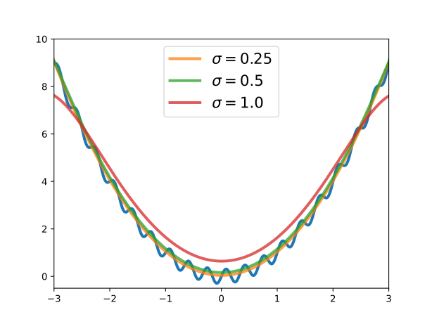
图 14.1:以采样并重新归一化后的高斯核对信号 f[t]:=t2+0.3sin⁡(6πt)f[t]\coloneqq t^{2}+0.3\sin(6\pi t) 进行平滑。Figure 14.1: Smoothing of the signal f[t]:=t2+0.3sin⁡(6πt)f[t]\coloneqq t^{2}+0.3\sin(6\pi t) with a sampled and renormalized Gaussian kernel.

14.1.4 求导Differentiation

值得注意的是,只要这两个函数及其导数均可积,卷积的导数便满足Remarkably, provided that the two functions are integrable with integrable derivatives, the derivative of the convolution satisfies

(f∗g)′=(f′∗g)=(f∗g′),(f\ast g)^{\prime}=(f^{\prime}\ast g)=(f\ast g^{\prime}),

这一等式只需在卷积的定义中交换求导与积分的次序即可得到。此外,还有如下命题。which simply stems from switching derivative and integral in the definition of the convolution. Moreover, we have the following proposition.

命题 14.1.2(卷积的可微性)。Proposition 14.1.2 (Differentiability of the convolution).
若 gg 在 R\mathbb{R} 上具有紧支集且 nn 次可微,而 ff 在 R\mathbb{R} 上局部可积,则 f∗gf\ast g 在 R\mathbb{R} 上 nn 次可微。If gg is nn-times differentiable with compact support over R\mathbb{R} and ff is locally integrable over R\mathbb{R}, then f∗gf\ast g is nn-times differentiable over R\mathbb{R}.

14.1.5 多维卷积Multidimensional convolution

至此,我们讨论的都是两个一元函数的卷积。该定义可以自然地推广到多元函数 f ⁣:RM→Rf\colon\mathbb{R}^{M}\to\mathbb{R} 与 g ⁣:RM→Rg\colon\mathbb{R}^{M}\to\mathbb{R},即So far, we studied the convolution of one-dimensional functions. The definition can be naturally extended to multidimensional functions f ⁣:RM→Rf\colon\mathbb{R}^{M}\to\mathbb{R} and g ⁣:RM→Rg\colon\mathbb{R}^{M}\to\mathbb{R} as

(f∗g)(μ):=∫RMf(u)g(μ−u) du,(f\ast g)({\bm{\mu}})\coloneqq\int_{\mathbb{R}^{M}}f({\bm{u}})g({\bm{\mu}}-{\bm{u}})\,d{\bm{u}},

这里同样假设积分存在。通常情况下,所用的高斯核其协方差矩阵为对角矩阵assuming again that the integral exists. Typically, a Gaussian kernel with diagonal covariance matrix is used

κσ(z)\displaystyle\kappa_{\sigma}({\bm{z}}) :=∏j=1M12πσje−12(zjσj)2=12πMσMe−12∥z∥22σ2,\displaystyle\coloneqq\prod_{j=1}^{M}\frac{1}{\sqrt{2\pi}\sigma_{j}}e^{-\frac{1}{2}(\frac{z_{j}}{\sigma_{j}})^{2}}=\frac{1}{\sqrt{2\pi}^{M}\sigma^{M}}e^{-\frac{1}{2}\frac{\|{\bm{z}}\|^{2}_{2}}{\sigma^{2}}}, (14.3)

其中第二个等式中假定了 σ1=⋯=σM\sigma_{1}=\dots=\sigma_{M}。在图像处理的语境下(此时 M=2M=2),该积分借助离散卷积来近似,所得结果称为高斯模糊。where, in the second equality, we assumed σ1=⋯=σM\sigma_{1}=\dots=\sigma_{M}. In an image processing context, where M=2M=2, it is approximated using a discrete convolution and it is called a Gaussian blur.

14.1.6 卷积与下确卷积之间的联系Link between convolution and infimal convolution

我们在 13.1 节中研究过的下确卷积,其形式为The infimal convolution we studied in Section 13.1 takes the form

(f□g)(μ):=inf⁡u∈RMf(u)+g(μ−u).(f\square g)({\bm{\mu}})\coloneqq\inf_{{\bm{u}}\in\mathbb{R}^{M}}f({\bm{u}})+g({\bm{\mu}}-{\bm{u}}).

作为对照,经典的卷积则取如下形式In comparison, the classical convolution takes the form

(F∗G)(μ):=∫RMF(u)G(μ−u) du.(F\ast G)({\bm{\mu}})\coloneqq\int_{\mathbb{R}^{M}}F({\bm{u}})G({\bm{\mu}}-{\bm{u}})\,d{\bm{u}}.

这两种卷积显然相互关联。下确卷积取的是下确界,并把 ff 与 gg 相加:它采用的是最小—加代数。经典卷积则执行积分,并将 FF 与 GG 相乘:它采用的是和—积代数。The two forms of convolution are clearly related. Infimal convolution performs an infimum and uses the sum of ff and gg: it uses a min-plus algebra. Classical convolution performs an integral and uses the product of FF and GG: it uses a sum-product algebra.

14.1.7 软下确卷积The soft infimal convolution

若在下确卷积的定义中以下确界换成软最小值,下确卷积与经典卷积之间的联系便会更加清晰。The link between the infimal convolution and the classical convolution can be further elucidated if we replace the infimum with a soft minimum in the definition of the infimal convolution.

定义 14.1.3(软下确卷积)。Definition 14.1.3 (Soft infimal convolution).
f ⁣:RM→Rf\colon\mathbb{R}^{M}\to\mathbb{R} 与 g ⁣:RM→Rg\colon\mathbb{R}^{M}\to\mathbb{R} 之间的软下确卷积定义为The soft infimal convolution between f ⁣:RM→Rf\colon\mathbb{R}^{M}\to\mathbb{R} and g ⁣:RM→Rg\colon\mathbb{R}^{M}\to\mathbb{R} is (f□εg)(μ):=softminεu∈RM f(u)+g(μ−u),(f\square_{\varepsilon}g)({\bm{\mu}})\coloneqq\underset{{\bm{u}}\in\mathbb{R}^{M}}{\mathrm{softmin}_{\varepsilon}} \ f({\bm{u}})+g({\bm{\mu}}-{\bm{u}}), 其中,对任意函数 h ⁣:S→Rh\colon\mathcal{S}\to\mathbb{R},我们将其在 S\mathcal{S} 上的软最小值(假设存在)定义为where we defined the soft minimum (assuming that it exists) over S\mathcal{S} of any function h ⁣:S→Rh\colon\mathcal{S}\to\mathbb{R} as softminεu∈S h(u):=−εlog⁡∫Sexp⁡(−h(u)/ε)du.\underset{{\bm{u}}\in\mathcal{S}}{\mathrm{softmin}_{\varepsilon}} \ h({\bm{u}})\coloneqq-\varepsilon\log\int_{\mathcal{S}}\exp\left(-h({\bm{u}})/\varepsilon\right)d{\bm{u}}.

我们便得到下确卷积,即 ε→0\varepsilon\to 0。We recover the infimal convolution as ε→0\varepsilon\to 0.

借助卷积进行计算Computation using a convolution

下面说明,软下确卷积可以用经典卷积改写。事实上,借助指数变量替换(在偏微分方程语境中有时称为 Cole-Hopf 变换),We now show that we can rewrite the soft infimal convolution using a classical convolution. Indeed, by using the exponential change of variable (sometimes referred to as Cole-Hopf transformation in a partial differential equation context)

Cε{f}(u)\displaystyle\mathcal{C}_{\varepsilon}\{f\}({\bm{u}}) :=exp⁡(−f(u)/ε)\displaystyle\coloneqq\exp(-f({\bm{u}})/\varepsilon)
Cε−1{F}(v)\displaystyle\mathcal{C}_{\varepsilon}^{-1}\{F\}({\bm{v}}) =−εlog⁡F(v),\displaystyle=-\varepsilon\log F({\bm{v}}),

我们可在指数域中定义每一个函数,we can define each function in the exponential domain,

Fε\displaystyle F_{\varepsilon} :=Cε{f}\displaystyle\coloneqq\mathcal{C}_{\varepsilon}\{f\}
Gε\displaystyle G_{\varepsilon} :=Cε{g}\displaystyle\coloneqq\mathcal{C}_{\varepsilon}\{g\}
Hε\displaystyle H_{\varepsilon} :=Cε{hε}.\displaystyle\coloneqq\mathcal{C}_{\varepsilon}\{h_{\varepsilon}\}.

容易验证,此时有It is easy to check that we then have

Hε(μ)=(Fε∗Gε)(μ).H_{\varepsilon}({\bm{\mu}})=(F_{\varepsilon}\ast G_{\varepsilon})({\bm{\mu}}).

回到对数域,便得到Back to log domain, we obtain

hε(μ)=Cε−1{Hε}(μ).h_{\varepsilon}({\bm{\mu}})=\mathcal{C}_{\varepsilon}^{-1}\{H_{\varepsilon}\}({\bm{\mu}}).

将该变换与其逆变换结合起来,可写成Combining the transformation and its inverse, we can write

hε(μ)=Cε−1{Cε{f}∗Cε{g}}(μ).\displaystyle h_{\varepsilon}({\bm{\mu}})=\mathcal{C}_{\varepsilon}^{-1}\{\mathcal{C}_{\varepsilon}\{f\}\ast\mathcal{C}_{\varepsilon}\{g\}\}({\bm{\mu}}).

以上结果表明,经过指数变量替换后,软下确卷积可化归为一次卷积的计算。这很有用,因为大小为 nn 的网格上的离散卷积可在 O(nlog⁡n)O(n\log n) 内算完。What we have shown is that, after an exponential change of variable, the soft infimal convolution can be reduced to the computation of a convolution. This is useful as a discrete convolution on a grid of size nn can be computed in O(nlog⁡n)O(n\log n).

14.1.8 软 Moreau 包络The soft Moreau envelope

我们在 13.1.2 节中看到,ff 与 R(z)=12z2R(z)=\frac{1}{2}z^{2} 之间的下确卷积即为 Moreau 包络,We saw in Section 13.1.2 that the infimal convolution between ff and R(z)=12z2R(z)=\frac{1}{2}z^{2} is the Moreau envelope,

Mf(μ):=(f□R)(μ)=inf⁡u∈RMf(u)+12∥μ−u∥22.M_{f}({\bm{\mu}})\coloneqq(f\square R)({\bm{\mu}})=\inf_{{\bm{u}}\in\mathbb{R}^{M}}f({\bm{u}})+\frac{1}{2}\|{\bm{\mu}}-{\bm{u}}\|^{2}_{2}.

将下确卷积替换为软下确卷积,便可定义“软”Moreau 包络,Replacing the infimal convolution with a soft infimal convolution, we can define the “soft” Moreau envelope,

Mfε(μ):=(f□εR)(μ)=softminεu∈RM f(u)+12∥μ−u∥22.M_{f}^{\varepsilon}({\bm{\mu}})\coloneqq(f\square_{\varepsilon}R)({\bm{\mu}})=\underset{{\bm{u}}\in\mathbb{R}^{M}}{\mathrm{softmin}_{\varepsilon}} \ f({\bm{u}})+\frac{1}{2}\|{\bm{\mu}}-{\bm{u}}\|^{2}_{2}.

需要强调,这一运算与 ff 同高斯核函数的卷积并不相同。事实上,有We emphasize that this operation is not the same as the convolution of ff with a Gaussian kernel. Indeed, we have

Mfε(μ)=−εlog⁡∫RMexp⁡((−f(u)−12∥μ−u∥22)/ε)du.\displaystyle M_{f}^{\varepsilon}({\bm{\mu}})=-\varepsilon\log\int_{\mathbb{R}^{M}}\exp\left((-f({\bm{u}})-\frac{1}{2}\|{\bm{\mu}}-{\bm{u}}\|_{2}^{2})/\varepsilon\right)d{\bm{u}}.

而while

(f∗κσ)(μ):=∫RMf(u)κσ(μ−u) du,\displaystyle(f\ast\kappa_{\sigma})({\bm{\mu}})\coloneqq\int_{\mathbb{R}^{M}}f({\bm{u}})\kappa_{\sigma}({\bm{\mu}}-{\bm{u}})\,d{\bm{u}},

其中 κσ\kappa_{\sigma} 例如由式 14.3 定义。where κσ\kappa_{\sigma} is for instance defined in Eq. 14.3.

我们已看到,Moreau 包络是光滑函数。那么,使用软 Moreau 包络究竟能带来什么好处?好处可能在于计算:软 Moreau 包络可用离散卷积来近似。We saw that the Moreau envelope is a smooth function. One may therefore ask what do we gain from using a soft Moreau envelope. The benefit can be computational, as the latter can be approximated using a discrete convolution.

14.2 Fourier 变换与 Laplace 变换14.2 Fourier and Laplace transforms

我们定义 ff 的 Fourier 变换为Let us define the Fourier transform of ff by

F(s):=F{f}(s):=∫−∞∞f(t)e−i2πst dt,s∈R.F(s)\coloneqq\mathcal{F}\{f\}(s)\coloneqq\int_{-\infty}^{\infty}f(t)e^{-i2\pi st}\,dt,\quad s\in\mathbb{R}.

注意,F{f}\mathcal{F}\{f\} 是一种函数变换:它将 ff 变为另一个函数 FF。Note that F{f}\mathcal{F}\{f\} is a function transformation: it transforms ff into another function FF.

14.2.1 卷积定理Convolution theorem

现在考虑卷积Now, consider the convolution

h(t):=(f∗g)(t).h(t)\coloneqq(f\ast g)(t).

若定义如下三个变换If we define the three transformations

F\displaystyle F :=F{f}, G:=F{g}, H:=F{h},\displaystyle\coloneqq\mathcal{F}\{f\},\ G\coloneqq\mathcal{F}\{g\},\ H\coloneqq\mathcal{F}\{h\},

卷积定理指出the convolution theorem states that

H(s)=F(s)⋅G(s),s∈R.H(s)=F(s)\cdot G(s),\quad s\in\mathbb{R}.

换一种写法,即有Written differently, we have

F{f∗g}=F{f}⋅F{g}.\mathcal{F}\{f\ast g\}=\mathcal{F}\{f\}\cdot\mathcal{F}\{g\}.

用文字来说,在 Fourier 域中,卷积运算变为乘法。反过来,In words, in the Fourier domain, the convolution operation becomes a multiplication. Conversely,

h(t)=(f∗g)(t)=F−1{F⋅G}(t),t∈R.h(t)=(f*g)(t)=\mathcal{F}^{-1}\{F\cdot G\}(t),\quad t\in\mathbb{R}.

若将 Fourier 变换替换为 Laplace 变换或双侧(双边)Laplace 变换,卷积定理同样成立。The convolution theorem also holds if we replace the Fourier transform with the Laplace transform or with the two-sided (bilateral) Laplace transform.

14.2.2 Fourier 变换与 Legendre 变换之间的联系Link between Fourier and Legendre transforms

在 13.2 节中,我们研究了另一种函数变换:凸共轭,又称 Legendre-Fenchel 变换。我们在表 14.1 中回顾了这些变换之间的类比关系。特别地,……的对应项In Section 13.2, we studied another function transformation: the convex conjugate, also known as Legendre-Fenchel transform. We recap the analogies between these transforms in Table 14.1. In particular, the counterpart of

F{f∗g}=F{f}⋅F{g}\mathcal{F}\{f\ast g\}=\mathcal{F}\{f\}\cdot\mathcal{F}\{g\}

对于下确卷积,与之对应的则是for the infimal convolution is

(f□g)∗=f∗+g∗.(f\square g)^{*}=f^{*}+g^{*}.

用文字来说,Legendre-Fenchel 变换之于下确卷积,恰如 Fourier 变换之于卷积。In words, the Legendre-Fenchel transform is to the infimal convolution what the Fourier transform is to the convolution.

表 14.1:Fourier 变换与 Legendre 变换之间的类比。更多共轭运算法则参见命题 13.2.6。Table 14.1: Analogy between Fourier and Legendre transforms. See Proposition 13.2.6 for more conjugate calculus rules.
Fourier F{f}\mathcal{F}\{f\}Fourier F{f}\mathcal{F}\{f\} Legendre f∗f^{*}Legendre f∗f^{*}
半环Semiring (+,⋅)(+,\cdot) (min⁡,+)(\min,+)
缩放 (a>0)(a>0)Scaling (a>0)(a>0) f(t)=g(t/a)f(t)=g(t/a) f(t)=ag(t/a)f(t)=ag(t/a)
F{f}(s)=aF{g}(as)\mathcal{F}\{f\}(s)=a\mathcal{F}\{g\}(as) f∗(s)=ag∗(s)f^{*}(s)=ag^{*}(s)
平移Translation f(t)=g(t−t0)f(t)=g(t-t_{0}) f(t)=g(t−t0)f(t)=g(t-t_{0})
F{f}(s)=e−i2πt0sF{g}(s)\mathcal{F}\{f\}(s)=e^{-i2\pi t_{0}s}\mathcal{F}\{g\}(s) f∗(s)=g∗(s)+t0f^{*}(s)=g^{*}(s)+t_{0}
卷积Convolution h=f∗gh=f\ast g h=f□gh=f\square g
F{h}=F{f}⋅F{g}\mathcal{F}\{h\}=\mathcal{F}\{f\}\cdot\mathcal{F}\{g\} h∗=f∗+g∗h^{*}=f^{*}+g^{*}
高斯/二次函数Gaussian / quadratic f(t)=e−at2f(t)=e^{-at^{2}} f(t)=a2t2f(t)=\frac{a}{2}t^{2}
F{f}(s)=πae−π2s2/a\mathcal{F}\{f\}(s)=\sqrt{\frac{\pi}{a}}e^{-\pi^{2}s^{2}/a} f∗(s)=12as2f^{*}(s)=\frac{1}{2a}s^{2}
平滑Smoothing f∗κσf\ast\kappa_{\sigma} f□12ε∥⋅∥22f\square\frac{1}{2\varepsilon}\|\cdot\|^{2}_{2}

14.2.3 软 Legendre-Fenchel 变换The soft Legendre-Fenchel transform

我们在 13.2 节中看到,函数 f ⁣:RM→Rf\colon\mathbb{R}^{M}\to\mathbb{R} 的 Legendre-Fenchel 变换(凸共轭)为We saw in Section 13.2 that the Legendre-Fenchel transform (convex conjugate) of a function f ⁣:RM→Rf\colon\mathbb{R}^{M}\to\mathbb{R} is

f∗(v):=max⁡u∈RM ⟨u,v⟩−f(u).f^{*}({\bm{v}})\coloneqq\max_{{\bm{u}}\in\mathbb{R}^{M}} \ \langle{\bm{u}},{\bm{v}}\rangle-f({\bm{u}}).

必要时,我们可以在 ff 的定义中加入一个指示函数来支持约束。该共轭可以通过 log-sum-exp 平滑化,后者起着软最大值的作用(13.5 节)。If necessary, we can support constraints by including an indicator function in the definition of ff. The conjugate can be smoothed out using a log-sum-exp, which plays the role of a soft maximum (Section 13.5).

定义 14.2.1(软凸共轭)。Definition 14.2.1 (Soft convex conjugate).
fε∗(v):=softmaxεu∈RM ⟨u,v⟩−f(u),f^{*}_{\varepsilon}({\bm{v}})\coloneqq\underset{{\bm{u}}\in\mathbb{R}^{M}}{\mathrm{softmax}_{\varepsilon}} \ \langle{\bm{u}},{\bm{v}}\rangle-f({\bm{u}}), 其中,对任意函数 g ⁣:S→Rg\colon\mathcal{S}\to\mathbb{R},我们将其在 S\mathcal{S} 上的软最大值(假设存在)定义为where we defined the soft maximum (assuming that it exists) over S\mathcal{S} of any function g ⁣:S→Rg\colon\mathcal{S}\to\mathbb{R} as softmaxεu∈S g(u):=εlog⁡∫Sexp⁡(g(u)/ε)du.\underset{{\bm{u}}\in\mathcal{S}}{\mathrm{softmax}_{\varepsilon}} \ g({\bm{u}})\coloneqq\varepsilon\log\int_{\mathcal{S}}\exp\left(g({\bm{u}})/\varepsilon\right)d{\bm{u}}.

在极限 ε→0\varepsilon\to 0 下,我们恢复凸共轭。In the limit ε→0\varepsilon\to 0, we recover the convex conjugate.

利用卷积进行计算Computation using a convolution

下面说明:若对 ff 施加双射变换,则该平滑后的共轭可以用卷积重写。We now show that this smoothed conjugate can be rewritten using a convolution if we apply a bijective transformation to ff.

命题 14.2.2(平滑凸共轭的卷积表示)。Proposition 14.2.2 (Smoothed convex conjugate as convolution).
平滑后的共轭可改写为The smoothed conjugate can be rewritten as fε∗(v)=Qε−1{1Qε{f}∗Gε}(v)f^{*}_{\varepsilon}({\bm{v}})=\mathcal{Q}_{\varepsilon}^{-1}\left\{\frac{1}{\mathcal{Q}_{\varepsilon}\{f\}\ast G_{\varepsilon}}\right\}\left({\bm{v}}\right) 其中where Gε\displaystyle G_{\varepsilon} :=Cε{12∥⋅∥22}=exp⁡(−12∥⋅∥22ε)\displaystyle\coloneqq\mathcal{C}_{\varepsilon}\left\{\frac{1}{2}\|\cdot\|^{2}_{2}\right\}=\exp\left(-\frac{1}{2}\frac{\|\cdot\|^{2}_{2}}{\varepsilon}\right) Qε{f}\displaystyle\mathcal{Q}_{\varepsilon}\{f\} :=Cε{f(⋅)−12∥⋅∥22}=exp⁡(12ε∥⋅∥22−1εf(⋅))\displaystyle\coloneqq\mathcal{C}_{\varepsilon}\left\{f(\cdot)-\frac{1}{2}\|\cdot\|^{2}_{2}\right\}=\exp\left(\frac{1}{2\varepsilon}\|\cdot\|^{2}_{2}-\frac{1}{\varepsilon}f(\cdot)\right) Qε−1{F}\displaystyle\mathcal{Q}_{\varepsilon}^{-1}\{F\} :=12∥⋅∥22−εlog⁡(F(⋅)).\displaystyle\coloneqq\frac{1}{2}\|\cdot\|^{2}_{2}-\varepsilon\log(F(\cdot)).

这一洞见由 Gabriel Peyré 于 2020 年 4 月发布在推特上。This insight was tweeted by Gabriel Peyré in April 2020.

证明 14.2.3。Proof 14.2.3.
fε∗(v)\displaystyle f^{\ast}_{\varepsilon}({\bm{v}}) :=εlog⁡∫exp⁡(1ε⟨u,v⟩−1εf(u))du\displaystyle\coloneqq\varepsilon\log\int\exp\left(\frac{1}{\varepsilon}\langle{\bm{u}},{\bm{v}}\rangle-\frac{1}{\varepsilon}f({\bm{u}})\right)d{\bm{u}}
=εlog⁡∫exp⁡(−12ε∥u−v∥22+12ε∥u∥22+12ε∥v∥22−1εf(u))du\displaystyle=\varepsilon\log\int\exp\left(-\frac{1}{2\varepsilon}\|{\bm{u}}-{\bm{v}}\|^{2}_{2}+\frac{1}{2\varepsilon}\|{\bm{u}}\|^{2}_{2}+\frac{1}{2\varepsilon}\|{\bm{v}}\|^{2}_{2}-\frac{1}{\varepsilon}f({\bm{u}})\right)d{\bm{u}}
=εlog⁡∫exp⁡(−12ε∥u−v∥22+12ε∥u∥22−1εf(u))du+12∥v∥22\displaystyle=\varepsilon\log\int\exp\left(-\frac{1}{2\varepsilon}\|{\bm{u}}-{\bm{v}}\|^{2}_{2}+\frac{1}{2\varepsilon}\|{\bm{u}}\|^{2}_{2}-\frac{1}{\varepsilon}f({\bm{u}})\right)d{\bm{u}}+\frac{1}{2}\|{\bm{v}}\|^{2}_{2}
=εlog⁡∫Gε(v−u)Qε{f}(u)du+12∥v∥22\displaystyle=\varepsilon\log\int G_{\varepsilon}({\bm{v}}-{\bm{u}})\mathcal{Q}_{\varepsilon}\{f\}({\bm{u}})d{\bm{u}}+\frac{1}{2}\|{\bm{v}}\|^{2}_{2}
=εlog⁡(Qε{f}∗Gε)(v)+12∥v∥22\displaystyle=\varepsilon\log(\mathcal{Q}_{\varepsilon}\{f\}\ast G_{\varepsilon})({\bm{v}})+\frac{1}{2}\|{\bm{v}}\|^{2}_{2}
=12∥v∥22−εlog⁡(1Qε{f}∗Gε)(v)\displaystyle=\frac{1}{2}\|{\bm{v}}\|^{2}_{2}-\varepsilon\log\left(\frac{1}{\mathcal{Q}_{\varepsilon}\{f\}\ast G_{\varepsilon}}\right)({\bm{v}})
=Qε−1{1Qε{f}∗Gε}(v)\displaystyle=\mathcal{Q}_{\varepsilon}^{-1}\left\{\frac{1}{\mathcal{Q}_{\varepsilon}\{f\}\ast G_{\varepsilon}}\right\}\left({\bm{v}}\right)
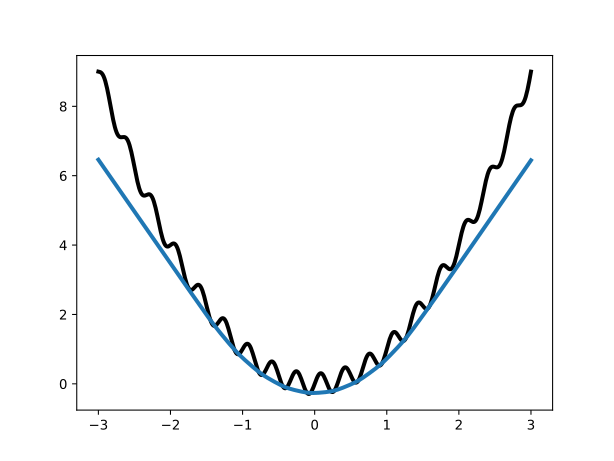
图 14.2:将平滑后的共轭应用两次,便得到函数的平滑双共轭(凸包络)。Figure 14.2: Applying the smoothed conjugate twice gives a smoothed biconjugate (convex envelope) of the function.

从这个视角我们能得到什么?凸共轭通常难以求得闭式形式。若把 RM\mathbb{R}^{M} 替换为离散集 S\mathcal{S}(即网格),我们便可以用离散卷积在 O(nlog⁡n)O(n\log n) 中近似平滑凸共轭,其中 n=∣S∣n=|\mathcal{S}|,What did we gain from this viewpoint? The convex conjugate can often be difficult to compute in closed form. If we replace RM\mathbb{R}^{M} with a discrete set S\mathcal{S} (i.e., a grid), we can then approximate the smoothed convex conjugate in O(nlog⁡n)O(n\log n), where n=∣S∣n=|\mathcal{S}|, using a discrete convolution,

(Qε{f}∗Gε)(v)\displaystyle(\mathcal{Q}_{\varepsilon}\{f\}\ast G_{\varepsilon})({\bm{v}}) ≈∑u∈SGε(v−u)Qε{f}(u)\displaystyle\approx\sum_{{\bm{u}}\in\mathcal{S}}G_{\varepsilon}({\bm{v}}-{\bm{u}})\mathcal{Q}_{\varepsilon}\{f\}({\bm{u}})
=Kq,\displaystyle={\bm{K}}{\bm{q}},

其中 K{\bm{K}} 是 n×nn\times n 高斯核矩阵,其元素对应 exp⁡(−12ε∥u−u′∥22)\exp(-\frac{1}{2\varepsilon}\|{\bm{u}}-{\bm{u}}^{\prime}\|^{2}_{2}),其中 u,u′∈S{\bm{u}},{\bm{u}}^{\prime}\in\mathcal{S};而 q{\bm{q}} 是 nn 维向量,其元素对应 exp⁡(1ε(12∥v∥22−f(u))\exp(\frac{1}{\varepsilon}(\frac{1}{2}\|{\bm{v}}\|^{2}_{2}-f({\bm{u}})),其中 u∈S{\bm{u}}\in\mathcal{S}。这为 13.2 节所讨论的快速 Legendre 变换算法提供了一种对 GPU 友好的替代方案。当然,由于维数灾难,该技术仅限于定义在低维集合上的函数。图 14.2 展示了将该技术用于计算函数的近似双共轭(凸包络)的情形。where K{\bm{K}} is the n×nn\times n Gaussian kernel matrix whose entries correspond to exp⁡(−12ε∥u−u′∥22)\exp(-\frac{1}{2\varepsilon}\|{\bm{u}}-{\bm{u}}^{\prime}\|^{2}_{2}) for u,u′∈S{\bm{u}},{\bm{u}}^{\prime}\in\mathcal{S} and q{\bm{q}} is the nn-dimensional vector whose entries correspond to exp⁡(1ε(12∥v∥22−f(u))\exp(\frac{1}{\varepsilon}(\frac{1}{2}\|{\bm{v}}\|^{2}_{2}-f({\bm{u}})) for u∈S{\bm{u}}\in\mathcal{S}. This provides a GPU-friendly alternative to the fast Legendre transform algorithm, discussed in Section 13.2. Of course, due to the curse of dimensionality, the technique is limited to functions defined on low-dimensional sets. We illustrate in Fig. 14.2 the application of the technique to computing an approximate biconjugate (convex envelope) of a function.

注 14.2.4(与双侧 Laplace 变换的联系)。Remark 14.2.4 (Link with the two-sided Laplace transform).
对于一维函数,我们也可以不借助卷积,而将软凸共轭写成For
one-dimensional functions, instead of using a convolution, we can also write the soft convex conjugate as
fε∗(v)\displaystyle f^{*}_{\varepsilon}(v) =εlog⁡∫−∞∞exp⁡(1ε[uv−f(u)]))du\displaystyle=\varepsilon\log\int_{-\infty}^{\infty}\exp\left(\frac{1}{\varepsilon}\left[uv-f(u)\right])\right)du =εlog⁡B{e−fε}(−vε)\displaystyle=\varepsilon\log\mathcal{B}\left\{e^{-\frac{f}{\varepsilon}}\right\}\left(-\frac{v}{\varepsilon}\right) =−Cε−1{B{Cε{f}}}(−vε)\displaystyle=-\mathcal{C}^{-1}_{\varepsilon}\left\{\mathcal{B}\left\{\mathcal{C}_{\varepsilon}\{f\}\right\}\right\}\left(-\frac{v}{\varepsilon}\right) 其中我们定义了双侧(双边)拉普拉斯变换where we defined the two-sided (bilateral) Laplace transform B{g}(v):=∫−∞∞e−uvg(u)du\mathcal{B}\{g\}(v)\coloneqq\int_{-\infty}^{\infty}e^{-uv}g(u)du 并假定该积分存在。and where we assumed that the integral exists.

14.3 示例14.3 Examples

本节回顾若干与高斯核的卷积具有解析解的实际例子。In this section, we review practical examples for which the convolution with a Gaussian kernel enjoys an analytical solution.

14.3.1 平滑的阶跃函数Smoothed step function

例 14.3.1(平滑的 Heaviside 函数)。Example 14.3.1 (Smoothed Heaviside).
Heaviside 阶跃函数定义为The Heaviside step function is defined by step(u):=h(u):={1 if u≥00 otherwise.\mathrm{step}(u)\coloneqq h(u)\coloneqq\begin{cases}1&\text{ if }u\geq 0\\ 0&\text{ otherwise}\end{cases}. 因此,取高斯核可得With the Gaussian kernel, we therefore obtain (h∗κσ)(μ)\displaystyle(h\ast\kappa_{\sigma})(\mu) =∫−∞μκσ(z)h(μ−z)dz+∫μ∞κσ(z)h(μ−z)dz\displaystyle=\int_{-\infty}^{\mu}\kappa_{\sigma}(z)h(\mu-z)dz+\int_{\mu}^{\infty}\kappa_{\sigma}(z)h(\mu-z)dz =∫−∞μκσ(z)dz\displaystyle=\int_{-\infty}^{\mu}\kappa_{\sigma}(z)dz =Φσ(μ)\displaystyle=\Phi_{\sigma}(\mu) =12[1+erf(μ2σ)],\displaystyle=\frac{1}{2}\left[1+\mathrm{erf}\left(\frac{\mu}{\sqrt{2}\sigma}\right)\right], 其中 Φσ(μ)\Phi_{\sigma}(\mu) 是均值为零、方差为 σ2\sigma^{2} 的高斯分布的 CDF,且此处用到了误差函数where Φσ(μ)\Phi_{\sigma}(\mu) is the CDF of the Gaussian distribution with zero mean and variance σ2\sigma^{2}, and where we used the error function erf⁡(z):=2π∫0ze−t2 dt,\operatorname{erf}(z)\coloneqq\frac{2}{\sqrt{\pi}}\int_{0}^{z}e^{-t^{2}}\,\mathrm{d}t, 我们两人此前都已在第 3 章中遇到过。误差函数虽然没有闭式表达式,但通常可在数值分析软件中直接调用,例如 SciPy。that we both already encountered in Chapter 3. Although there is no closed form for the error function, it is commonly available in numerical analysis software, such as SciPy.

14.3.2 平滑的 ReLU 函数Smoothed ReLU function

例 14.3.2(平滑的 ReLU)。Example 14.3.2 (Smoothed ReLU).
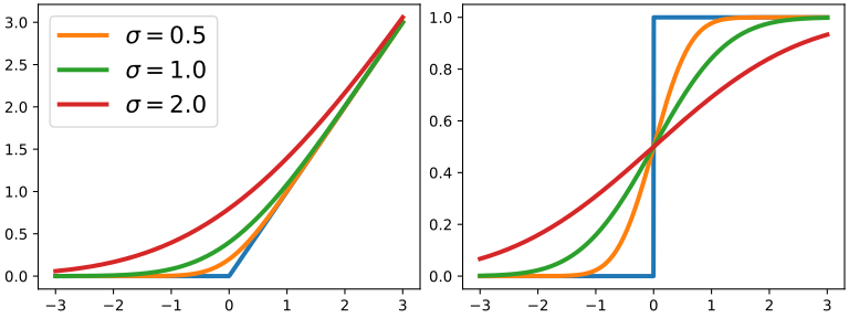
ReLU 定义为The ReLU is defined by r(u):={u if u≥00 otherwise=u⋅h(u).r(u)\coloneqq\begin{cases}u&\text{ if }u\geq 0\\ 0&\text{ otherwise}\end{cases}=u\cdot h(u). 与前一例类似,可得Similarly to the previous example, we obtain (r∗κσ)(μ)\displaystyle(r\ast\kappa_{\sigma})(\mu) =∫−∞μκσ(z)r(μ−z)dz\displaystyle=\int_{-\infty}^{\mu}\kappa_{\sigma}(z)r(\mu-z)dz =∫−∞μκσ(z)(μ−z)dz\displaystyle=\int_{-\infty}^{\mu}\kappa_{\sigma}(z)(\mu-z)dz =μ∫−∞μκσ(z)dz−∫−∞μκσ(z)zdz\displaystyle=\mu\int_{-\infty}^{\mu}\kappa_{\sigma}(z)dz-\int_{-\infty}^{\mu}\kappa_{\sigma}(z)zdz =μΦσ(μ)+σ2κσ(μ).\displaystyle=\mu\Phi_{\sigma}(\mu)+\sigma^{2}\kappa_{\sigma}(\mu). 在第二个积分中,令 a:=12σ2a\coloneqq\frac{1}{2\sigma^{2}},我们用到In the second integral, setting a:=12σ2a\coloneqq\frac{1}{2\sigma^{2}}, we used ∫ze−az2dz=−12a∫etdt=−12aet+C=−12ae−az2+C\int ze^{-az^{2}}dz=-\frac{1}{2a}\int e^{t}dt=-\frac{1}{2a}e^{t}+C=-\frac{1}{2a}e^{-az^{2}}+C 以及 t:=−az2⇒zdz=−12adtt\coloneqq-az^{2}\Rightarrow zdz=-\frac{1}{2a}dt。and t:=−az2⇒zdz=−12adtt\coloneqq-az^{2}\Rightarrow zdz=-\frac{1}{2a}dt.
图 14.3:通过与高斯核卷积对 ReLU 和 Heaviside 函数进行平滑,图中给出宽度 σ\sigma 的三个取值。Figure 14.3: Smoothing of the ReLU and Heaviside functions by convolution with a Gaussian kernel, for three values of the width σ\sigma.

为说明卷积的求导,我们展示如何对平滑的 ReLU 求导。To illustrate differentiation of the convolution, we show how to differentiate the smoothed ReLU.

例 14.3.3(对平滑的 ReLU 求导)。Example 14.3.3 (Differentiating the smoothed ReLU).
对例 14.3.2 中的平滑 ReLU 求导,可得Differentiating the smoothed ReLU from Example 14.3.2, we obtain (r∗κσ)′=(r′∗κσ)=h∗κσ=Φσ.(r\ast\kappa_{\sigma})^{\prime}=(r^{\prime}\ast\kappa_{\sigma})=h\ast\kappa_{\sigma}=\Phi_{\sigma}. 因此,平滑 ReLU 的导数为平滑的 Heaviside 阶跃函数,这并不出人意料。再次求导,可得,Therefore, unsurprisingly, the derivative of the smoothed ReLU is the smoothed Heaviside step function. Differentiating once again, we obtain, (r∗κσ)′′=(h∗κσ)′=(h′∗κσ)=δ∗κσ=κσ,(r\ast\kappa_{\sigma})^{\prime\prime}=(h\ast\kappa_{\sigma})^{\prime}=(h^{\prime}\ast\kappa_{\sigma})=\delta\ast\kappa_{\sigma}=\kappa_{\sigma}, 其中导数 h′h^{\prime} 几乎处处有良定义。利用 h∗κσ=Φσh\ast\kappa_{\sigma}=\Phi_{\sigma} 和 Φσ′=κσ\Phi_{\sigma}^{\prime}=\kappa_{\sigma} 也可得到同一结果,因为 Φσ\Phi_{\sigma} 和 κσ\kappa_{\sigma} 分别是均值为零、方差为 σ2\sigma^{2} 的高斯分布的 CDF 与 PDF。where the derivative h′h^{\prime} is well-defined almost everywhere. We can arrive at the same result by using that h∗κσ=Φσh\ast\kappa_{\sigma}=\Phi_{\sigma} and Φσ′=κσ\Phi_{\sigma}^{\prime}=\kappa_{\sigma}, since Φσ\Phi_{\sigma} and κσ\kappa_{\sigma} are the CDF and PDF of the Gaussian with zero mean and σ2\sigma^{2} variance.

14.4 黑箱函数的扰动14.4 Perturbation of blackbox functions

本节回顾如何利用蒙特卡洛估计近似计算与核函数的卷积及其梯度。In this section, we review how to approximately compute a convolution with a kernel and its gradient using Monte-Carlo estimation.

14.4.1 位置—尺度族中的期望Expectation in a location-scale family

平滑函数 f:RM→Rf:\mathbb{R}^{M}\rightarrow\mathbb{R} 的一个相当直观的做法,是让输入 μ{\bm{\mu}} 受到服从某个噪声分布 pp 的加性噪声 Z∼pZ\sim p 的扰动,再对其取值取平均。由此定义替代函数A rather intuitive approach to smooth a function f:RM→Rf:\mathbb{R}^{M}\rightarrow\mathbb{R} is to average its values on an input μ{\bm{\mu}}, perturbed by some additive noise Z∼pZ\sim p, for some noise distribution pp. This defines the surrogate

fσ(μ):=EZ∼p[f(μ+σZ)].f_{\sigma}({\bm{\mu}})\coloneqq\mathbb{E}_{Z\sim p}[f({\bm{\mu}}+\sigma Z)].

参数 σ\sigma 控制扰动强度:当 σ→0\sigma\rightarrow 0 时,我们自然回到 ff。若定义变换(变量替换),则可得到等价的视角The parameter σ\sigma controls the perturbation strength: as σ→0\sigma\rightarrow 0, we naturally recover ff. An equivalent viewpoint is obtained by defining the transformation (change of variables)

U:=μ+σZ.U\coloneqq{\bm{\mu}}+\sigma Z.

于是有We then have

U∼pμ,σ,U\sim p_{{\bm{\mu}},\sigma},

其中 pμ,σp_{{\bm{\mu}},\sigma} 是由噪声分布 pp 生成的位置族分布,即 ZZ 经该变换得到的前推分布(见 12.4.4 节)。在此记号下,初始噪声分布 pp 就简单地是 p=p0,1p=p_{{\mathbf{0}},1}。由此,扰动后的函数可从这两个视角表示为where pμ,σp_{{\bm{\mu}},\sigma} is the location-family distribution generated by the noise distribution pp. It is the pushforward distribution of ZZ through the transformation (see Section 12.4.4). In this notation, the initial noise distribution pp is then simply p=p0,1p=p_{{\mathbf{0}},1}. The perturbed function can then be expressed from these two perspectives as

fσ(μ)\displaystyle f_{\sigma}({\bm{\mu}}) =EZ∼p0,1[f(μ+σ⋅Z)]\displaystyle=\mathbb{E}_{Z\sim p_{{\mathbf{0}},1}}[f({\bm{\mu}}+\sigma\cdot Z)]
=EU∼pμ,σ[f(U)].\displaystyle=\mathbb{E}_{U\sim p_{{\bm{\mu}},\sigma}}[f(U)]. (14.4)

将期望写成概率密度函数的积分,便自然得到前文所述通过卷积实现的平滑Writing the expectation as the integral of a p.d.f, we naturally recover the smoothing by convolution presented earlier,

fσ(μ)\displaystyle f_{\sigma}({\bm{\mu}}) =∫f(μ+σz)p0,1(z)dz\displaystyle=\int f({\bm{\mu}}+\sigma{\bm{z}})p_{{\mathbf{0}},1}({\bm{z}})d{\bm{z}}
=f∗κσ(μ),\displaystyle=f\ast\kappa_{\sigma}({\bm{\mu}}),

其中我们定义了核函数where we defined the kernel

κσ(z):=p0,σ(−z).\kappa_{\sigma}({\bm{z}})\coloneqq p_{{\mathbf{0}},\sigma}(-{\bm{z}}).

在下文中,我们假设噪声分布可分解为In the sequel, we assume that the noise distribution decomposes as

p0,1(z):=exp⁡(−ν(z))/C,p_{{\mathbf{0}},1}({\bm{z}})\coloneqq\exp(-\nu({\bm{z}}))/C,

其中 ν(z)\nu({\bm{z}}) 是噪声分布的对数密度,CC 是归一化常数。例如,取 ν(z)=12∥z∥22\nu({\bm{z}})=\frac{1}{2}\|{\bm{z}}\|^{2}_{2}、C=2πMC=\sqrt{2\pi}^{M},即得到具有对角协方差矩阵的高斯分布及相应的高斯核。where ν(z)\nu({\bm{z}}) is the log-density of the noise distribution and CC is a normalization constant. For instance, the Gaussian distribution with diagonal covariance matrix and the corresponding Gaussian kernel are obtained with ν(z)=12∥z∥22\nu({\bm{z}})=\frac{1}{2}\|{\bm{z}}\|^{2}_{2} and C=2πMC=\sqrt{2\pi}^{M}.

用蒙特卡洛估计进行近似Approximation by Monte-Carlo estimation

14.1.3 节的做法是在网格上用离散卷积近似上述积分(连续卷积);与之不同,期望视角提示我们可用蒙特卡洛估计来估计 fσ(μ)f_{\sigma}({\bm{\mu}}):只需从该分布中抽取样本,在这些样本处对函数求值,再取平均。除单纯的蒙特卡洛估计外,[42] 还研究了更精细的近似方案。Instead of approximating the integral above (continuous convolution) with a discrete convolution on a grid, as we did in Section 14.1.3, the expectation perspective suggests that we can estimate fσ(μ)f_{\sigma}({\bm{\mu}}) by Monte-Carlo estimation: we simply draw samples from the distribution, evaluate the function at these samples and average. Beyond mere Monte-Carlo estimation, more elaborate approximation schemes are studied in [42].

14.4.2 通过重参数化进行梯度估计Gradient estimation by reparametrization

只要交换求导与积分次序的条件成立(见 12.1 节),就有Provided that the conditions for swapping differentiation and integration hold (see Section 12.1), we have

∇fσ(μ)=EZ∼p0,1[∇f(μ+σ⋅Z)].\nabla f_{\sigma}({\bm{\mu}})=\mathbb{E}_{Z\sim p_{{\mathbf{0}},1}}[\nabla f({\bm{\mu}}+\sigma\cdot Z)]. (14.5)

注意,若 ff 只是几乎处处可微,该公式仍可能成立。例如,当 ff 为 ReLU 时,∇f\nabla f 为 Heaviside 阶跃函数,用上述公式即可得到 fσf_{\sigma} 的正确梯度;见例 14.3.1。然而,若 ff 并非绝对连续,该公式可能不成立。例如,当 ff 为 Heaviside 函数时,(14.5) 的右端为 0,与 fσf_{\sigma} 的梯度不符;仍见例 14.3.1。Note that if ff is only differentiable almost everywhere, the formula may still hold. For example, if ff is the ReLU, then ∇f\nabla f is the Heaviside step function, and we obtain the correct gradient of fσf_{\sigma} using the formula above; see Example 14.3.1. However, if ff is not absolutely continuous, the formula may not hold. For example, if ff is the Heaviside function, the right-hand side of (14.5) is 0 which does not match the gradient of fσf_{\sigma}; see again Example 14.3.1.

从 (14.4) 中 fσf_{\sigma} 的第二个表达式可以看出,(14.5) 中的梯度公式可视为一种重参数化技巧 U=μ+σZU={\bm{\mu}}+\sigma Z;见 12.4 节。也就是说,有From the second expression of fσf_{\sigma} in (14.4), we can see the formula of the gradient in (14.5) as a reparametrization trick U=μ+σZU={\bm{\mu}}+\sigma Z; see Section 12.4. Namely, we have

∇fσ(μ)\displaystyle\nabla f_{\sigma}({\bm{\mu}}) =∇μEU∼pμ,σ[f(U)]\displaystyle=\nabla_{\bm{\mu}}\mathbb{E}_{U\sim p_{{\bm{\mu}},\sigma}}[f(U)]
=∇μEZ∼p0,1[f(μ+σ⋅Z)]\displaystyle=\nabla_{\bm{\mu}}\mathbb{E}_{Z\sim p_{{\mathbf{0}},1}}[f({\bm{\mu}}+\sigma\cdot Z)]
=EZ∼p0,1[∇μf(μ+σ⋅Z)]\displaystyle=\mathbb{E}_{Z\sim p_{{\mathbf{0}},1}}[\nabla_{\bm{\mu}}f({\bm{\mu}}+\sigma\cdot Z)]
=EZ∼p0,1[∇f(μ+σ⋅Z)].\displaystyle=\mathbb{E}_{Z\sim p_{{\mathbf{0}},1}}[\nabla f({\bm{\mu}}+\sigma\cdot Z)]. (14.6)

14.4.3 用 SFE 与 Stein 引理进行梯度估计Gradient estimation by SFE, Stein’s lemma

某些情况下,我们可能无法获得 ∇f\nabla f,或者 ff 未必绝对连续,因而 (14.5) 中的公式无法适用。遇到这类情形,可以改用 12.3 节介绍的得分函数估计量(SFE)。此处,对于 fσ(μ)=EU∼pμ,σ[f(U)]f_{\sigma}({\bm{\mu}})=\mathbb{E}_{U\sim p_{{\bm{\mu}},\sigma}}[f(U)],我们得到In some cases, we may not have access to ∇f\nabla f or ff may not be absolutely continuous and therefore the formula in (14.5) cannot apply. For these cases, we can use the score function estimator (SFE) from Section 12.3. Here, for fσ(μ)=EU∼pμ,σ[f(U)]f_{\sigma}({\bm{\mu}})=\mathbb{E}_{U\sim p_{{\bm{\mu}},\sigma}}[f(U)], we obtain

∇fσ(μ)=EU∼pμ,σ[f(U)∇μlog⁡pμ,σ(U)].\nabla f_{\sigma}({\bm{\mu}})=\mathbb{E}_{U\sim p_{{\bm{\mu}},\sigma}}[f(U)\nabla_{{\bm{\mu}}}\log p_{{\bm{\mu}},\sigma}(U)].

由于 PDF 可以写成Since the PDF can be written as

pμ,σ(u)=1σp0,1((u−μ)/σ),p_{{\bm{\mu}},\sigma}({\bm{u}})=\frac{1}{\sigma}p_{{\mathbf{0}},1}(({\bm{u}}-{\bm{\mu}})/\sigma),

其中where

p0,1(z):=exp⁡(−ν(z))/C,p_{{\mathbf{0}},1}({\bm{z}})\coloneqq\exp(-\nu({\bm{z}}))/C,

于是得到we obtain

∇μlog⁡pμ,σ(u)=∇ν((u−μ)/σ)/σ.\nabla_{\bm{\mu}}\log p_{{\bm{\mu}},\sigma}({\bm{u}})=\nabla\nu(({\bm{u}}-{\bm{\mu}})/\sigma)/\sigma.

综上,我们已证明To summarize, we have shown that

∇fσ(μ)\displaystyle\nabla f_{\sigma}({\bm{\mu}}) =EU∼pμ,σ[f(U)∇ν((U−μ)/σ)/σ]\displaystyle=\mathbb{E}_{U\sim p_{{\bm{\mu}},\sigma}}[f(U)\nabla\nu((U-{\bm{\mu}})/\sigma)/\sigma]
=EZ∼p0,1[f(μ+σ⋅Z)∇ν(Z)/σ],\displaystyle=\mathbb{E}_{Z\sim p_{{\mathbf{0}},1}}[f({\bm{\mu}}+\sigma\cdot Z)\nabla\nu(Z)/\sigma], (14.7)

其中使用了变量替换 Z=(U−μ)/σZ=(U-{\bm{\mu}})/\sigma。这一技巧同样适用于估计关于 θ=(μ,σ){\bm{\theta}}=({\bm{\mu}},\sigma) 的梯度,或估计向量值函数之期望的雅可比矩阵。where we used the change of variable Z=(U−μ)/σZ=(U-{\bm{\mu}})/\sigma. The same technique can also be used if we want to estimate the gradient w.r.t. θ=(μ,σ){\bm{\theta}}=({\bm{\mu}},\sigma) or if we want to estimate the Jacobian of the expectation of a vector-valued function.

在高斯噪声这一特殊情形下,由于 ∇ν(z)=z\nabla\nu({\bm{z}})={\bm{z}},可得In the particular case of Gaussian noise, since ∇ν(z)=z\nabla\nu({\bm{z}})={\bm{z}}, we obtain

∇fσ(μ)\displaystyle\nabla f_{\sigma}({\bm{\mu}}) =EZ∼p0,1[f(μ+σ⋅Z)Z/σ].\displaystyle=\mathbb{E}_{Z\sim p_{{\mathbf{0}},1}}[f({\bm{\mu}}+\sigma\cdot Z)Z/\sigma].

这被称为 Stein 引理。需要指出,上式是平滑后函数 fσf_{\sigma} 的梯度的无偏估计量;但对于原始函数 ff 的梯度(假设该梯度存在),它却是有偏估计量。不过,平滑通常有益,因为它能加速基于梯度的算法的收敛。关于扰动后的一般程序的梯度计算,[111] 已有详细研究。This is known as Stein’s lemma. It should be noted that the above is an unbiased estimator of the gradient of the smoothed function fσf_{\sigma}, but a biased estimator of the gradient of the original function ff (assuming that it exists). However, smoothing is usually a good thing, as it can accelerate the convergence of gradient-based algorithms. Computing the gradient of perturbed general programs is studied in detail in [111].

14.4.4 重参数化与 SFE 之间的联系Link between reparametrization and SFE

利用对数导数恒等式,对任意具有可微密度 pp 的分布,有Using the log-derivative identity, we have for any distribution with differentiable density pp

EZ∼p[h(Z)∇log⁡p(Z)]\displaystyle\mathbb{E}_{Z\sim p}[h(Z)\nabla\log p(Z)] =∫RMh(z)(∇p(z)p(z))p(z)dz\displaystyle=\int_{\mathbb{R}^{M}}h({\bm{z}})\left(\frac{\nabla p({\bm{z}})}{p({\bm{z}})}\right)p({\bm{z}})d{\bm{z}}
=∫RMh(z)∇p(z)dz.\displaystyle=\int_{\mathbb{R}^{M}}h({\bm{z}})\nabla p({\bm{z}})d{\bm{z}}.

利用分部积分,并假设当 ∥z∥→∞\|{\bm{z}}\|\to\infty 时 h(z)p(z)h({\bm{z}})p({\bm{z}}) 趋于零,可得Using integration by parts and assuming that h(z)p(z)h({\bm{z}})p({\bm{z}}) goes to zero when ∥z∥→∞\|{\bm{z}}\|\to\infty, we have

∫RMh(z)∇p(z)dz=−∫RMp(z)∇h(z)dz.\int_{\mathbb{R}^{M}}h({\bm{z}})\nabla p({\bm{z}})d{\bm{z}}=-\int_{\mathbb{R}^{M}}p({\bm{z}})\nabla h({\bm{z}})d{\bm{z}}.

由此得到恒等式We have therefore the identity

EZ∼p[h(Z)∇log⁡p(Z)]=−EZ∼p[∇h(Z)].\mathbb{E}_{Z\sim p}[h(Z)\nabla\log p(Z)]=-\mathbb{E}_{Z\sim p}[\nabla h(Z)].

重要的是,与 12.3 节的 SFE 估计量不同,该恒等式使用的是关于 z{\bm{z}} 的梯度,而非关于分布参数的梯度。不过,借助重参数化 h(z):=f(μ+σ⋅z)h({\bm{z}})\coloneqq f({\bm{\mu}}+\sigma\cdot{\bm{z}}),有 ∇h(z)=∇f(μ+σ⋅z)⋅σ\nabla h({\bm{z}})=\nabla f({\bm{\mu}}+\sigma\cdot{\bm{z}})\cdot\sigma,从而Importantly, contrary to the SFE estimator from Section 12.3, this identity uses gradients with respect to z{\bm{z}}, not with respect to the parameters of the distribution. Nevertheless, using the reparametrization h(z):=f(μ+σ⋅z)h({\bm{z}})\coloneqq f({\bm{\mu}}+\sigma\cdot{\bm{z}}), we have ∇h(z)=∇f(μ+σ⋅z)⋅σ\nabla h({\bm{z}})=\nabla f({\bm{\mu}}+\sigma\cdot{\bm{z}})\cdot\sigma so that

∇fσ(μ)\displaystyle\nabla f_{\sigma}({\bm{\mu}}) =∇μEU∼pμ,σ[f(U)]\displaystyle=\nabla_{\bm{\mu}}\mathbb{E}_{U\sim p_{{\bm{\mu}},\sigma}}[f(U)]
=EZ∼p0,1[∇f(μ+σ⋅Z)](reparametrization trick)\displaystyle=\mathbb{E}_{Z\sim p_{{\mathbf{0}},1}}[\nabla f({\bm{\mu}}+\sigma\cdot Z)]\quad\text{(reparametrization trick)}
=EZ∼p0,1[∇h(Z)/σ]\displaystyle=\mathbb{E}_{Z\sim p_{{\mathbf{0}},1}}[\nabla h(Z)/\sigma]
=−EZ∼p0,1[h(Z)∇log⁡p(Z)/σ]\displaystyle=-\mathbb{E}_{Z\sim p_{{\mathbf{0}},1}}[h(Z)\nabla\log p(Z)/\sigma]
=EZ∼p0,1[h(Z)∇ν(Z)/σ]\displaystyle=\mathbb{E}_{Z\sim p_{{\mathbf{0}},1}}[h(Z)\nabla\nu(Z)/\sigma]
=EZ∼p0,1[f(μ+σ⋅Z)∇ν(Z)/σ](score function estimator)\displaystyle=\mathbb{E}_{Z\sim p_{{\mathbf{0}},1}}[f({\bm{\mu}}+\sigma\cdot Z)\nabla\nu(Z)/\sigma]\quad\text{(score function estimator)}

本质上,分部积分使我们能够把重参数化技巧估计量转化为 SFE 估计量。关于分部积分在机器学习中的更多应用,参见 Francis Bach 的精彩博客文章。Essentially, integration by parts allowed us to convert the reparametrization trick estimator into the SFE estimator. For more applications of integration by parts in machine learning, see Francis Bach’s excellent blog post.

14.4.5 方差缩减与进化策略Variance reduction and evolution strategies

如第 12 章所述,SFE 的方差偏大。现在我们对其应用方差缩减技术。为此,假设对于 Z∼p0,1Z\sim p_{{\mathbf{0}},1},∇ν(Z)\nabla\nu(Z) 的均值为零。例如,这一假设对高斯噪声成立。该假设意味着As discussed in Chapter 12, the SFE suffers from high variance. We now apply variance reduction techniques to it. To do so, we assume that ∇ν(Z)\nabla\nu(Z) has zero mean for Z∼p0,1Z\sim p_{{\mathbf{0}},1}. This assumption for example holds for Gaussian noise. This assumption implies that

EZ∼p0,1[f(μ)∇ν(Z)/σ]=f(μ)EZ∼p0,1[∇ν(Z)/σ]=0\mathbb{E}_{Z\sim p_{{\mathbf{0}},1}}[f({\bm{\mu}})\nabla\nu(Z)/\sigma]=f({\bm{\mu}})\mathbb{E}_{Z\sim p_{{\mathbf{0}},1}}[\nabla\nu(Z)/\sigma]={\mathbf{0}}

因而and therefore

∇fσ(μ)=EZ∼p0,1[(f(μ+σ⋅Z)−f(μ))∇ν(Z)/σ].\nabla f_{\sigma}({\bm{\mu}})=\mathbb{E}_{Z\sim p_{{\mathbf{0}},1}}\left[(f({\bm{\mu}}+\sigma\cdot Z)-f({\bm{\mu}}))\nabla\nu(Z)/\sigma\right]. (14.8)

这是 12.3 节所述控制变量的一个例子。它可以理解为:用有限差分来计算沿随机方向 ZZ 的方向导数(见下文“极限情形”)。受中心有限差分的启发,我们还可以使用This is an example of control variate discussed in Section 12.3. This can be interpreted as using a finite difference for computing a directional derivative in the random direction ZZ (see “limit case” below). Inspired by a central finite difference, we can also use

∇fσ(μ)=EZ∼p0,1[(f(μ+σ⋅Z)−f(μ−σ⋅Z))∇ν(Z)/(2σ)].\nabla f_{\sigma}({\bm{\mu}})=\mathbb{E}_{Z\sim p_{{\mathbf{0}},1}}\left[(f({\bm{\mu}}+\sigma\cdot Z)-f({\bm{\mu}}-\sigma\cdot Z))\nabla\nu(Z)/(2\sigma)\right]. (14.9)

这些估计量已被用于黑箱(零阶)优化算法,例如进化策略 [173] 或随机无梯度优化 [147]。对于二次函数,容易证明第二个估计量的方差更低 [167]。同时采样 ZZ 与 −Z-Z 的思想被称为对偶采样(antithetic)[76] 或镜像采样(mirrored sampling)[36]。进化策略也被用于获得部分展开计算图的无偏梯度估计量 [202]。在图 14.4 中,我们实验比较了带方差缩减与不带方差缩减的 SFE 在黑箱梯度估计上的表现。These estimators have been used as part of blackbox (zero-order) optimization algorithms, such as evolution strategies [173] or random gradient-free optimization [147]. For quadratic functions, it is easy to show that the second estimator achieves lower variance [167]. The idea of sampling both ZZ and −Z-Z simultaneously is called antithetic [76] or mirrored sampling [36]. Evolution strategies have also been used to obtain unbiased gradient estimators of partially unrolled computational graphs [202]. We empirically compare the SFE with or without variance reduction for blackbox gradient estimation in Fig. 14.4.
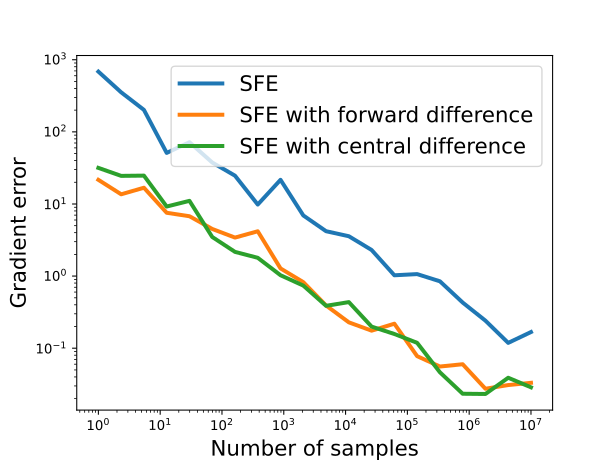
图 14.4:带方差缩减与不带方差缩减的得分函数估计量(SFE)在黑箱梯度估计上的比较。图中给出 ∣∇f(μ)−∇fσ(μ)∣|\nabla f(\mu)-\nabla f_{\sigma}(\mu)| 在 f(u):=u3f(u)\coloneqq u^{3} 和 fσ(μ):=E[f(μ+σZ)]f_{\sigma}(\mu)\coloneqq\mathbb{E}[f(\mu+\sigma Z)] 时的误差,其中 Z∼Normal(0,1)Z\sim\mathrm{Normal}(0,1),σ:=0.1\sigma\coloneqq 0.1。为估计 ∇fσ(μ)\nabla f_{\sigma}(\mu),我们比较了三个估计量:朴素 SFE,即式 14.7;采用前向差分且已做方差缩减的 SFE 估计量,即式 14.8;以及采用中心差分且已做方差缩减的 SFE 估计量,即式 14.9。在这三种情形中,我们都用一定数量的样本通过蒙特卡洛估计来近似期望。方差缩减后的估计量不仅误差更小,而且当 σ\sigma 变小时在数值上也更稳定。Figure 14.4: Comparison of the score function estimator (SFE) with or without variance reduction for blackbox gradient estimation. We show the error ∣∇f(μ)−∇fσ(μ)∣|\nabla f(\mu)-\nabla f_{\sigma}(\mu)| for f(u):=u3f(u)\coloneqq u^{3} and fσ(μ):=E[f(μ+σZ)]f_{\sigma}(\mu)\coloneqq\mathbb{E}[f(\mu+\sigma Z)], where Z∼Normal(0,1)Z\sim\mathrm{Normal}(0,1) and σ:=0.1\sigma\coloneqq 0.1. To estimate ∇fσ(μ)\nabla f_{\sigma}(\mu), we compare three estimators: the vanilla SFE Eq. 14.7, the SFE estimator with forward difference (variance reduced) Eq. 14.8, and the SFE estimator with central difference (variance reduced) Eq. 14.9. In all three cases, we approximate the expectation by Monte-Carlo estimation using some number of samples. The variance-reduced estimators not only achieve smaller error, they are also more numerically stable as σ\sigma gets smaller.

14.4.6 零温度极限Zero-temperature limit

现在讨论极限情形 σ→0\sigma\to 0。也就是说,我们假设不希望进行平滑,并且 ∇f\nabla f 存在。回顾可知,ff 在 μ{\bm{\mu}} 处沿方向 z{\bm{z}} 的方向导数为We now discuss the limit case σ→0\sigma\to 0. That is, we assume that we do not want to perform smoothing and that ∇f\nabla f exists. We recall that the directional derivative of ff at μ{\bm{\mu}} in the direction z{\bm{z}} is

∂f(μ)[z]\displaystyle\partial f({\bm{\mu}})[{\bm{z}}] =⟨∇f(μ),z⟩\displaystyle=\langle\nabla f({\bm{\mu}}),{\bm{z}}\rangle
=lim⁡σ→0[f(μ+σ⋅z)−f(μ)]/σ.\displaystyle=\lim_{\sigma\to 0}\left[f({\bm{\mu}}+\sigma\cdot{\bm{z}})-f({\bm{\mu}})\right]/\sigma.

当 σ→0\sigma\to 0 且 ZZ 服从标准高斯分布,即 ∇ν(z)=z\nabla\nu({\bm{z}})={\bm{z}} 时,式 14.8 因而变为When σ→0\sigma\to 0 and ZZ follows the standard Gaussian distribution, meaning that ∇ν(z)=z\nabla\nu({\bm{z}})={\bm{z}}, Eq. 14.8 therefore becomes

∇fσ(μ)\displaystyle\nabla f_{\sigma}({\bm{\mu}}) =EZ∼p0,1[∂f(μ)[Z]∇ν(Z)]\displaystyle=\mathbb{E}_{Z\sim p_{{\mathbf{0}},1}}\left[\partial f({\bm{\mu}})[Z]\nabla\nu(Z)\right]
=EZ∼p0,1[∂f(μ)[Z]Z]\displaystyle=\mathbb{E}_{Z\sim p_{{\mathbf{0}},1}}\left[\partial f({\bm{\mu}})[Z]Z\right]
=EZ∼p0,1[⟨∇f(μ),Z⟩Z]\displaystyle=\mathbb{E}_{Z\sim p_{{\mathbf{0}},1}}\left[\langle\nabla f({\bm{\mu}}),Z\rangle Z\right]
=EZ∼p0,1[ZZ⊤∇f(μ)]\displaystyle=\mathbb{E}_{Z\sim p_{{\mathbf{0}},1}}\left[ZZ^{\top}\nabla f({\bm{\mu}})\right]
=∇f(μ).\displaystyle=\nabla f({\bm{\mu}}).

这并不应太令人意外,因为从卷积的视角我们已经知道,当 σ→0\sigma\to 0 时 fσ(μ)=(f∗κσ)(μ)→f(μ)f_{\sigma}({\bm{\mu}})=(f\ast\kappa_{\sigma})({\bm{\mu}})\to f({\bm{\mu}})。这重新得到了 8.7 节中已经给出的随机化前向模式估计量。This should not be too surprising, as we already know from the convolution perspective that fσ(μ)=(f∗κσ)(μ)→f(μ)f_{\sigma}({\bm{\mu}})=(f\ast\kappa_{\sigma})({\bm{\mu}})\to f({\bm{\mu}}) when σ→0\sigma\to 0. This recovers the randomized forward-mode estimator already presented in Section 8.7.

14.5 Gumbel 技巧14.5 Gumbel tricks

14.5.1 Gumbel 分布The Gumbel distribution

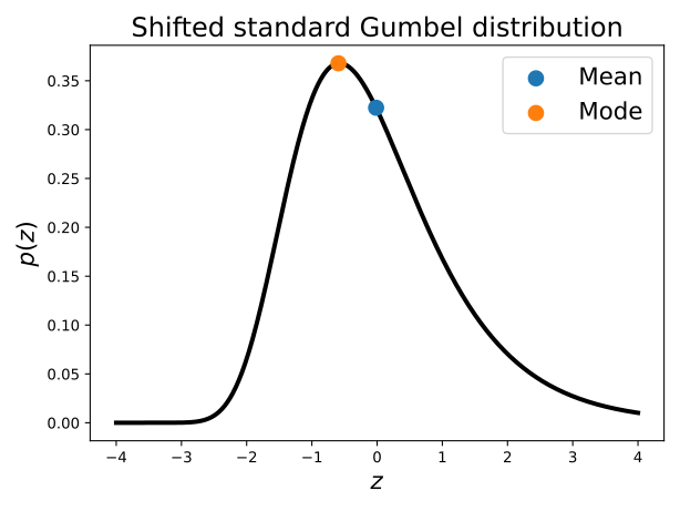
Gumbel 分布是极值理论中经常使用的一种分布。如图 14.5 所示,我们考虑平移后的标准 Gumbel 分布,其 PDF 定义为The Gumbel distribution is a distribution frequently used in extreme value theory. As illustrated in Fig. 14.5, we consider the shifted standard Gumbel distribution, whose PDF is defined by

p(z):=exp⁡(−ν(z)),p(z)\coloneqq\exp(-\nu(z)),

其中where

ν(z):=z+γ+exp⁡(−(z+γ)),\nu(z)\coloneqq z+\gamma+\exp(-(z+\gamma)),

并且其中 γ≈0.577\gamma\approx 0.577 是欧拉常数。注意,在某些表述中,该分布不做平移,即不加上 γ\gamma。若 ZZ 服从平移后的标准 Gumbel 分布,我们记作 Z∼Gumbel(0,1)Z\sim\mathrm{Gumbel}(0,1)。and where γ≈0.577\gamma\approx 0.577 is Euler’s constant. Note that in some formulations, the distribution is not shifted, i.e., γ\gamma is not added. If ZZ is distributed according to the shifted standard Gumbel distribution, we write Z∼Gumbel(0,1)Z\sim\mathrm{Gumbel}(0,1).

为得到带有位置—尺度参数 μ{\bm{\mu}} 与 σ\sigma 的多元推广,我们取 MM 个独立随机变量 Z:=(Z1,…,ZM)Z\coloneqq(Z_{1},\ldots,Z_{M}),并施加位置—尺度变换(12.4.1 节)。即,To obtain a multivariate extension with location-scale parameters μ{\bm{\mu}} and σ\sigma, we take MM independent random variables Z:=(Z1,…,ZM)Z\coloneqq(Z_{1},\ldots,Z_{M}) and apply the location-scale transform (Section 12.4.1). That is,

U∼Gumbel(μ,σ)  ⟺  U=μ+σZ, Zi∼Gumbel(0,1).U\sim\mathrm{Gumbel}({\bm{\mu}},\sigma)\iff U={\bm{\mu}}+\sigma Z, \ Z_{i}\sim\mathrm{Gumbel}(0,1).

由于我们采用的是平移后的标准 Gumbel 分布,自然得到 E[U]=μ\mathbb{E}[U]={\bm{\mu}} 与 Var⁡(U)=σ2\operatorname{Var}(U)=\sigma^{2}。我们可以用 Gumbel 噪声替代 14.4 节中所用的高斯噪声。所幸,在特定情形下,我们能够以闭式形式计算扰动函数的期望。As we used shifted standard Gumbel distributions, we naturally get that E[U]=μ\mathbb{E}[U]={\bm{\mu}} and Var⁡(U)=σ2\operatorname{Var}(U)=\sigma^{2}. We can use Gumbel noise as an alternative to the Gaussian noise used in Section 14.4. Thankfully, in particular cases, we can compute closed-form expressions of the expectation of perturbed functions.

注 14.5.1(Gumbel 分布与指数分布之间的联系)。Remark 14.5.1 (Link between Gumbel and exponential distribution).
随机变量 ZZ 服从 Gumbel⁡(μ,1)\operatorname{Gumbel}(\mu,1) 分布,当且仅当 exp⁡(−Z)\exp(-Z) 服从指数分布 Exp⁡(exp⁡(μ−γ))\operatorname{Exp}(\exp(\mu-\gamma))。要看出这一点,只需计算 exp⁡(−Z)\exp(-Z) 的 CDF,并认出它正是 Exp⁡(exp⁡(μ−γ))\operatorname{Exp}(\exp(\mu-\gamma)) 的 CDF。因此,在比较 Gumbel 分布时,我们可以利用指数分布的标准性质。A random variable ZZ is distributed as Gumbel⁡(μ,1)\operatorname{Gumbel}(\mu,1) if and only if exp⁡(−Z)\exp(-Z) is distributed as an exponential distribution Exp⁡(exp⁡(μ−γ))\operatorname{Exp}(\exp(\mu-\gamma)). To see this, one can simply compute the CDF of exp⁡(−Z)\exp(-Z) and recognize the CDF of Exp⁡(exp⁡(μ−γ))\operatorname{Exp}(\exp(\mu-\gamma)). Therefore, when comparing Gumbel distributions, we can use standard properties of the exponential distribution.
注 14.5.2(采样 Gumbel 噪声)。Remark 14.5.2 (Sampling Gumbel noise).
若 U∼Uniform(0,1)U\sim\mathrm{Uniform}(0,1),则 Z:=−log⁡(−log⁡(U))−γZ\coloneqq-\log(-\log(U))-\gamma 满足 Z∼Gumbel(0,1)Z\sim\mathrm{Gumbel}(0,1);这里我们回顾到,Gumbel(0,1)\mathrm{Gumbel}(0,1) 表示平移后的标准 Gumbel 分布。要看出这一点,只需注意 P(Z≤t)=P(U≤exp⁡(exp⁡(−(γ+t))))=exp⁡(exp⁡(−(γ+t)))\mathbb{P}(Z\leq t)=\mathbb{P}(U\leq\exp(\exp(-(\gamma+t))))=\exp(\exp(-(\gamma+t))),而其中最后一个表达式正是 Gumbel(0,1)\mathrm{Gumbel}(0,1) 的 CDF。If U∼Uniform(0,1)U\sim\mathrm{Uniform}(0,1), then Z:=−log⁡(−log⁡(U))−γZ\coloneqq-\log(-\log(U))-\gamma satisfies Z∼Gumbel(0,1)Z\sim\mathrm{Gumbel}(0,1), where we recall that we use Gumbel(0,1)\mathrm{Gumbel}(0,1) to denote the shifted standard Gumbel distribution. To see this, note that P(Z≤t)=P(U≤exp⁡(exp⁡(−(γ+t))))=exp⁡(exp⁡(−(γ+t)))\mathbb{P}(Z\leq t)=\mathbb{P}(U\leq\exp(\exp(-(\gamma+t))))=\exp(\exp(-(\gamma+t))), where the last expression matches the CDF of Gumbel(0,1)\mathrm{Gumbel}(0,1).
图 14.5:我们采用平移后的标准 Gumbel 分布定义,使均值在 z=0z=0 处取得,众数在 z=−γz=-\gamma 处取得。若采用未平移的定义,则均值与众数将分别在 γ\gamma 与 00 处取得。Figure 14.5: We use a shifted definition of the standard Gumbel distribution so that the mean is achieved at z=0z=0, and the mode at z=−γz=-\gamma. With an unshifted definition, the mean and the mode would be achieved at γ\gamma and 00, respectively.

14.5.2 扰动的比较Perturbed comparison

首先,Gumbel 分布可用于平滑二值比较,例如大于或等于运算符。回顾后者,对任意 μ1,μ2∈R\mu_{1},\mu_{2}\in\mathbb{R},其定义为To start with, the Gumbel distribution can be used to smooth a binary comparison like the greater than or equal operators. Recall that the latter is defined for any μ1,μ2∈R\mu_{1},\mu_{2}\in\mathbb{R} as

gt(μ1,μ2):={1if μ1≥μ20if μ1<μ2=step(μ1−μ2),\mathrm{gt}(\mu_{1},\mu_{2})\coloneqq\begin{cases}1&\text{if}\ \mu_{1}\geq\mu_{2}\\ 0&\text{if}\ \mu_{1}<\mu_{2}\end{cases}=\mathrm{step}(\mu_{1}-\mu_{2}),

其中 step\mathrm{step} 是 Heaviside 函数。如下文所示,用 Gumbel 噪声扰动每个变量,我们便能重新得到 logistic(a−b)=1/(1+e−(a−b))\mathrm{logistic}(a-b)=1/(1+e^{-(a-b)}),作为 step(a−b)\mathrm{step}(a-b) 的近似。where step\mathrm{step} is the Heaviside function. As shown below, by perturbing each variable with Gumbel noise, we recover logistic(a−b)=1/(1+e−(a−b))\mathrm{logistic}(a-b)=1/(1+e^{-(a-b)}) as an approximation of step(a−b)\mathrm{step}(a-b).

命题 14.5.3(二值变量的 Gumbel 技巧)。Proposition 14.5.3 (Gumbel trick for binary variables).
设 Z1,Z2∼Gumbel(0,1)Z_{1},Z_{2}\sim\mathrm{Gumbel}(0,1) 为两个独立随机变量。它们经位置—尺度变换(第 12.4.1 节)后的差服从 logistic 分布(注 3.3.1),即Let
Z1,Z2∼Gumbel(0,1)Z_{1},Z_{2}\sim\mathrm{Gumbel}(0,1) be two independent random variables. The difference of their location-scale transform (Section 12.4.1) is distributed according to a logistic distribution (Remark 3.3.1), i.e.,
μ1+σZ1−(μ2+σZ2)∼Logistic(μ1−μ2,σ),\mu_{1}+\sigma Z_{1}-(\mu_{2}+\sigma Z_{2})\sim\mathrm{Logistic}(\mu_{1}-\mu_{2},\sigma), 其中 μ1,μ2∈R\mu_{1},\mu_{2}\in\mathbb{R},σ>0\sigma>0。特别地,有for μ1,μ2∈R\mu_{1},\mu_{2}\in\mathbb{R} and σ>0\sigma>0. In particular, we have EZ1,Z2[gt(μ1+σZ1,μ2+σZ2)]=11+e−(μ1−μ2)/σ.\mathbb{E}_{Z_{1},Z_{2}}[\mathrm{gt}(\mu_{1}+\sigma Z_{1},\mu_{2}+\sigma Z_{2})]=\frac{1}{1+e^{-(\mu_{1}-\mu_{2})/\sigma}}.
证明 14.5.4。Proof 14.5.4.

我们首先推导 μ1+σZ1−(μ2+σZ2)\mu_{1}+\sigma Z_{1}-(\mu_{2}+\sigma Z_{2}) 的 CDF,如下:We first derive the CDF of μ1+σZ1−(μ2+σZ2)\mu_{1}+\sigma Z_{1}-(\mu_{2}+\sigma Z_{2}) as

P(μ1+σZ1−(μ2+σZ2)≤t)\displaystyle\mathbb{P}(\mu_{1}+\sigma Z_{1}-(\mu_{2}+\sigma Z_{2})\leq t) =P(μ1/σ+Z1≤(μ2+t)/σ+Z2)\displaystyle=\mathbb{P}\left(\mu_{1}/\sigma+Z_{1}\leq(\mu_{2}+t)/\sigma+Z_{2}\right)
=P(e−(μ1/σ+Z1)≥e−((μ2+t)/σ+Z2)).\displaystyle=\mathbb{P}\left(e^{-(\mu_{1}/\sigma+Z_{1})}\geq e^{-((\mu_{2}+t)/\sigma+Z_{2})}\right).

根据注 14.5.1,有 e−(μ1/σ+Z1)∼Exp⁡(exp⁡(μ1/σ−γ))e^{-(\mu_{1}/\sigma+Z_{1})}\sim\operatorname{Exp}(\exp(\mu_{1}/\sigma-\gamma)),对 e−(μ2+t)/σ+Z2e^{-(\mu_{2}+t)/\sigma+Z_{2}} 同理。此时容易证明,若 U∼Exp⁡(u),V∼Exp⁡(v)U\sim\operatorname{Exp}(u),V\sim\operatorname{Exp}(v) 相互独立,则 P(U≤V)=u/(u+v)\mathbb{P}(U\leq V)=u/(u+v)。因此,我们得到By Remark 14.5.1, e−(μ1/σ+Z1)∼Exp⁡(exp⁡(μ1/σ−γ))e^{-(\mu_{1}/\sigma+Z_{1})}\sim\operatorname{Exp}(\exp(\mu_{1}/\sigma-\gamma)), and similarly for e−(μ2+t)/σ+Z2e^{-(\mu_{2}+t)/\sigma+Z_{2}}. Now one easily shows that if U∼Exp⁡(u),V∼Exp⁡(v)U\sim\operatorname{Exp}(u),V\sim\operatorname{Exp}(v) independent, then P(U≤V)=u/(u+v)\mathbb{P}(U\leq V)=u/(u+v). Hence, we get

P(μ1+σZ1−(μ2+σZ2)≤t)\displaystyle\mathbb{P}(\mu_{1}+\sigma Z_{1}-(\mu_{2}+\sigma Z_{2})\leq t) =e(μ2+t)/σ−γe(μ2+t)/σ−γ+eμ1/σ−γ\displaystyle=\frac{e^{(\mu_{2}+t)/\sigma-\gamma}}{e^{(\mu_{2}+t)/\sigma-\gamma}+e^{\mu_{1}/\sigma-\gamma}}
=11+e−(t−(μ1−μ2))/σ.\displaystyle=\frac{1}{1+e^{-(t-(\mu_{1}-\mu_{2}))/\sigma}}.

我们认出,这正是均值为 μ1−μ2\mu_{1}-\mu_{2}、尺度为 σ\sigma 的 logistic 分布的 CDF,记作 Logistic(μ1−μ2,σ)\mathrm{Logistic}(\mu_{1}-\mu_{2},\sigma)。至于最后一个论断,我们只需有We recognize the CDF of the logistic distribution with mean μ1−μ2\mu_{1}-\mu_{2} and scale σ\sigma, denoted Logistic(μ1−μ2,σ)\mathrm{Logistic}(\mu_{1}-\mu_{2},\sigma). For the last claim, we simply have that

E[gt(μ1+σZ1,μ2+σZ2)]\displaystyle\mathbb{E}[\mathrm{gt}(\mu_{1}+\sigma Z_{1},\mu_{2}+\sigma Z_{2})] =E[step(μ1+σZ1−(μ2+σZ2))]\displaystyle=\mathbb{E}\left[\mathrm{step}(\mu_{1}+\sigma Z_{1}-(\mu_{2}+\sigma Z_{2}))\right]
=P(μ1+σZ1−(μ2+σZ2)≥0)\displaystyle=\mathbb{P}(\mu_{1}+\sigma Z_{1}-(\mu_{2}+\sigma Z_{2})\geq 0)
=11+e−(μ1−μ2)/σ.\displaystyle=\frac{1}{1+e^{-(\mu_{1}-\mu_{2})/\sigma}}.

14.5.3 扰动的 argmaxPerturbed argmax

假设我们想要平滑Suppose we want to smooth

y(u):=arg max⁡y∈{e1,…,eM}⟨y,u⟩=ϕ(i(u)),{\bm{y}}({\bm{u}})\coloneqq\argmax_{{\bm{y}}\in\{{\bm{e}}_{1},\dots,{\bm{e}}_{M}\}}\langle{\bm{y}},{\bm{u}}\rangle=\phi(i({\bm{u}})),

其中where

i(u)\displaystyle i({\bm{u}}) :=arg max⁡i∈[M]ui\displaystyle\coloneqq\argmax_{i\in[M]}u_{i}
ϕ(i)\displaystyle\phi(i) :=ei\displaystyle\coloneqq{\bm{e}}_{i}

其中 ϕ(i)\phi(i) 是 i∈[M]i\in[M] 的 one-hot 编码。结果表明,用 Gumbel 噪声扰动后的函数 y(u){\bm{y}}({\bm{u}}) 具有闭式期望,而它正是 softargmax。where ϕ(i)\phi(i) is the one-hot encoding of i∈[M]i\in[M]. It turns out that the function y(u){\bm{y}}({\bm{u}}) perturbed using Gumbel noise enjoys a closed form expectation, which is nothing else than the softargmax.

命题 14.5.5(分类变量的 Gumbel 技巧)。Proposition 14.5.5 (Gumbel trick for categorical variables).
设 MM 为独立随机变量 Z∼Gumbel(0,1)∈RMZ\sim\mathrm{Gumbel}({\mathbf{0}},1)\in\mathbb{R}^{M}。则对 μ∈RM{\bm{\mu}}\in\mathbb{R}^{M} 与 σ>0\sigma>0,Let us define MM independent random variables Z∼Gumbel(0,1)∈RMZ\sim\mathrm{Gumbel}({\mathbf{0}},1)\in\mathbb{R}^{M}. Then, for μ∈RM{\bm{\mu}}\in\mathbb{R}^{M} and σ>0\sigma>0, Y:=i(μ+σ⋅Z)  ⟹  Y∼Categorical(softargmax(μ/σ)).Y\coloneqq i({\bm{\mu}}+\sigma\cdot Z)\implies Y\sim\mathrm{Categorical}(\mathrm{softargmax}({\bm{\mu}}/\sigma)). 此外,有Moreover, we have yσ(μ)\displaystyle{\bm{y}}_{\sigma}({\bm{\mu}}) =EZ[y(μ+σ⋅Z)]\displaystyle=\mathbb{E}_{Z}[{\bm{y}}({\bm{\mu}}+\sigma\cdot Z)] =EY[ϕ(Y)]\displaystyle=\mathbb{E}_{Y}[\phi(Y)] =softargmax(μ/σ).\displaystyle=\mathrm{softargmax}({\bm{\mu}}/\sigma).
证明 14.5.6。Proof 14.5.6.

对于 k∈[M]k\in[M],我们有For k∈[M]k\in[M], we have that

P(Y=k)\displaystyle\mathbb{P}(Y=k) =P(arg max⁡i∈[M]{μi+σZi}=k)\displaystyle=\mathbb{P}\left(\argmax_{i\in[M]}\{\mu_{i}+\sigma Z_{i}\}=k\right)
=P(arg min⁡i∈[M]{e−μi/σ−Zi}=k)\displaystyle=\mathbb{P}\left(\argmin_{i\in[M]}\{e^{-\mu_{i}/\sigma-Z_{i}}\}=k\right)

由注 14.5.1 可知,e−μi/σ−Zi∼Exp⁡(exp⁡(μi/σ−γ))e^{-\mu_{i}/\sigma-Z_{i}}\sim\operatorname{Exp}(\exp(\mu_{i}/\sigma-\gamma))。作为练习,读者不难验证:对于参数为 u1,…,uMu_{1},\ldots,u_{M} 的 U1,…,UMU_{1},\ldots,U_{M} 个独立指数随机变量,有 P(arg min⁡i∈[M]{Ui}=k)=uk/∑i=1Mui\mathbb{P}(\argmin_{i\in[M]}\{U_{i}\}=k)=u_{k}/\sum_{i=1}^{M}u_{i}。由此得到By Remark 14.5.1, we have that e−μi/σ−Zi∼Exp⁡(exp⁡(μi/σ−γ))e^{-\mu_{i}/\sigma-Z_{i}}\sim\operatorname{Exp}(\exp(\mu_{i}/\sigma-\gamma)). One easily verifies as an exercise, that, for U1,…,UMU_{1},\ldots,U_{M} independent exponential variables with parameters u1,…,uMu_{1},\ldots,u_{M}, we have P(arg min⁡i∈[M]{Ui}=k)=uk/∑i=1Mui\mathbb{P}(\argmin_{i\in[M]}\{U_{i}\}=k)=u_{k}/\sum_{i=1}^{M}u_{i}. Hence, we get

P(Y=k)=exp⁡(μk/σ)∑i=1Mexp⁡(μi/σ),\mathbb{P}(Y=k)=\frac{\exp(\mu_{k}/\sigma)}{\sum_{i=1}^{M}\exp(\mu_{i}/\sigma)},

即that is,

Y∼Categorical(softargmax(μ/σ)).Y\sim\mathrm{Categorical}(\mathrm{softargmax}({\bm{\mu}}/\sigma)).

最后一个论断可由 YY 的分布以及 ϕ\phi 的定义推出。The last claim follows from the distribution of YY and the definition of ϕ\phi.

14.5.4 扰动的 maxPerturbed max

若我们此时扰动的是 max 而非 argmax,也有类似的结果。A similar result holds if we now wish to perturb the max instead of the argmax.

命题 14.5.7(与 log-sum-exp 的联系)。Proposition 14.5.7 (Link to log-sum-exp).
设 MM 为独立随机变量 Z∼Gumbel(0,1)∈RMZ\sim\mathrm{Gumbel}({\mathbf{0}},1)\in\mathbb{R}^{M},并且Let us define MM independent random variables Z∼Gumbel(0,1)∈RMZ\sim\mathrm{Gumbel}({\mathbf{0}},1)\in\mathbb{R}^{M} and f(u):=max⁡i∈[M]ui.f({\bm{u}})\coloneqq\max_{i\in[M]}u_{i}. 则对 μ∈RM{\bm{\mu}}\in\mathbb{R}^{M} 与 σ>0\sigma>0,Then, for μ∈RM{\bm{\mu}}\in\mathbb{R}^{M} and σ>0\sigma>0, V:=f(μ+σ⋅Z)  ⟹  V∼Gumbel(σLSE(μ/σ),σ).V\coloneqq f({\bm{\mu}}+\sigma\cdot Z)\implies V\sim\mathrm{Gumbel}(\sigma\mathrm{LSE}({\bm{\mu}}/\sigma),\sigma). 此外,有Moreover, we have fσ(μ):=EZ[f(μ+σ⋅Z)]=EV[V]=σ⋅LSE(μ/σ).f_{\sigma}({\bm{\mu}})\coloneqq\mathbb{E}_{Z}[f({\bm{\mu}}+\sigma\cdot Z)]=\mathbb{E}_{V}[V]=\sigma\cdot\mathrm{LSE}({\bm{\mu}}/\sigma).
证明 14.5.8。Proof 14.5.8.

我们按如下方式推导 f(μ+σ⋅Z)f({\bm{\mu}}+\sigma\cdot Z) 的累积分布函数:We derive the CDF of f(μ+σ⋅Z)f({\bm{\mu}}+\sigma\cdot Z) as

P(max⁡i∈[M]{μi+σZi}≤t)\displaystyle\mathbb{P}(\max_{i\in[M]}\{\mu_{i}+\sigma Z_{i}\}\leq t) =P(min⁡i∈[M]{e−(μi/σ−Zi)}≥e−t/σ)\displaystyle=\mathbb{P}\left(\min_{i\in[M]}\{e^{-(\mu_{i}/\sigma-Z_{i})}\}\geq e^{-t/\sigma}\right)

我们有 e−(μi/σ−Zi)∼Exp⁡(exp⁡(μi/σ)−γ)e^{-(\mu_{i}/\sigma-Z_{i})}\sim\operatorname{Exp}(\exp(\mu_{i}/\sigma)-\gamma);而参数为 uiu_{i} 的 U1,…,UMU_{1},\ldots,U_{M} 个独立指数随机变量满足 min⁡i∈[M]Ui∼Exp⁡(∑i=1Mui)\min_{i\in[M]}U_{i}\sim\operatorname{Exp}(\sum_{i=1}^{M}u_{i})。因此,We have e−(μi/σ−Zi)∼Exp⁡(exp⁡(μi/σ)−γ)e^{-(\mu_{i}/\sigma-Z_{i})}\sim\operatorname{Exp}(\exp(\mu_{i}/\sigma)-\gamma) and for U1,…,UMU_{1},\ldots,U_{M} independent exponential random variables with parameters uiu_{i}, we have min⁡i∈[M]Ui∼Exp⁡(∑i=1Mui)\min_{i\in[M]}U_{i}\sim\operatorname{Exp}(\sum_{i=1}^{M}u_{i}). Hence,

P(max⁡i∈[M]{μi+σZi}≤t)\displaystyle\mathbb{P}\left(\max_{i\in[M]}\{\mu_{i}+\sigma Z_{i}\}\leq t\right) =exp⁡(−∑i=1M(exp⁡(μi/σ−γ))exp⁡(−t/σ))\displaystyle=\exp\left(-\sum_{i=1}^{M}(\exp(\mu_{i}/\sigma-\gamma))\exp(-t/\sigma)\right)
=exp⁡(−exp⁡(−(t−σLSE(μ/σ))/σ−γ)).\displaystyle=\exp(-\exp(-(t-\sigma\mathrm{LSE}({\bm{\mu}}/\sigma))/\sigma-\gamma)).

我们认出,这正是位置—尺度参数为 σLSE(μ/σ)\sigma\mathrm{LSE}({\bm{\mu}}/\sigma) 与 σ\sigma 的平移 Gumbel 分布的累积分布函数。We recognize the CDF of the shifted Gumbel distribution with location-scale parameters σLSE(μ/σ)\sigma\mathrm{LSE}({\bm{\mu}}/\sigma) and σ\sigma.

关于 Gumbel 技巧的延伸阅读,可参见 Tim Vieira 的精彩博客。For further reading on the Gumbel trick, see Tim Vieira’s great blog.

14.5.5 用于采样的 Gumbel 技巧Gumbel trick for sampling

Gumbel 技巧本身也可用于采样,且无需计算 softargmax 的归一化常数。事实上,命题 14.5.5 保证:若 ZZ 为 Gumbel 噪声,则 YY 服从 Categorical(softargmax(μ/σ))\mathrm{Categorical}(\mathrm{softargmax}({\bm{\mu}}/\sigma)) 分布。计算 YY 所需的 arg-max 运算可一趟完成。因此,我们得到一种一趟算法,可直接从 logits μ{\bm{\mu}} 中采样,而无需显式计算概率 softargmax(μ/σ)\mathrm{softargmax}({\bm{\mu}}/\sigma)。The Gumbel trick is also useful in its own right for sampling without computing the normalization constant of the softargmax. Indeed, Proposition 14.5.5 ensures that if ZZ is Gumbel noise, then YY is distributed according to Categorical(softargmax(μ/σ))\mathrm{Categorical}(\mathrm{softargmax}({\bm{\mu}}/\sigma)). Computing the arg-maximum, as required to compute YY, can be done in one pass. Therefore, we obtain a one-pass algorithm to sample directly from the logits μ{\bm{\mu}}, without explicitly computing the probabilities softargmax(μ/σ)\mathrm{softargmax}({\bm{\mu}}/\sigma).

人们或许会问,这种技巧是否也能用于正态分布。遗憾的是,此时并不存在闭式形式,因为这需要对 M−1M-1 个高斯分布的最大值的累积分布函数进行积分。不过,还可以定义其他技巧,例如使用 Weibull 分布,参见 [10]。One may wonder whether such trick could also be used with the normal distribution. Unfortunately, there is no closed form in this case because it would require integrating the CDF of the maximum of M−1M-1 Gaussian distributions. However, other tricks can be defined such as using Weibull distributions, see [10].

14.5.6 扰动与 MAPPerturb-and-MAP

此前,我们在分类设定下讨论了 Gumbel 技巧,其中 Y=[M]\mathcal{Y}=[M]。在结构化预测设定中,输出通常嵌入于 RM\mathbb{R}^{M} 之中,但输出空间极为庞大。也就是说,Y⊆RM\mathcal{Y}\subseteq\mathbb{R}^{M},但 ∣Y∣≫M|\mathcal{Y}|\gg M。随后,结构化输出借助最大后验(MAP)oracle 进行解码Previously, we discussed the Gumbel trick in the classification setting, where Y=[M]\mathcal{Y}=[M]. In the structured prediction setting, outputs are typically embedded in RM\mathbb{R}^{M} but the output space is very large. That is, Y⊆RM\mathcal{Y}\subseteq\mathbb{R}^{M} but ∣Y∣≫M|\mathcal{Y}|\gg M. Structured outputs are then decoded using a maximum a-posteriori (MAP) oracle

f(u)\displaystyle f({\bm{u}}) :=max⁡y∈Y⟨y,u⟩\displaystyle\coloneqq\max_{{\bm{y}}\in\mathcal{Y}}\langle{\bm{y}},{\bm{u}}\rangle
y(u)\displaystyle{\bm{y}}({\bm{u}}) :=arg max⁡y∈Y⟨y,u⟩.\displaystyle\coloneqq\argmax_{{\bm{y}}\in\mathcal{Y}}\langle{\bm{y}},{\bm{u}}\rangle.

在这一设定下,ff 与 y{\bm{y}} 的扰动版本,For this setting, the perturbed versions of ff and y{\bm{y}},

fσ(μ)\displaystyle f_{\sigma}({\bm{\mu}}) :=EZ[f(μ+σ⋅Z)]\displaystyle\coloneqq\mathbb{E}_{Z}[f({\bm{\mu}}+\sigma\cdot Z)]
yσ(μ)\displaystyle{\bm{y}}_{\sigma}({\bm{\mu}}) :=EZ[y(μ+σ⋅Z)],\displaystyle\coloneqq\mathbb{E}_{Z}[{\bm{y}}({\bm{\mu}}+\sigma\cdot Z)],

一般不再具有闭式形式。不过,我们可以借助蒙特卡洛估计对它们作近似。对于 ∇fσ(μ)\nabla f_{\sigma}({\bm{\mu}}) 的梯度,存在两种估计量 [2, 23]。no longer enjoy a closed form in general. However, we can approximate them using Monte-carlo estimation. For the gradient of ∇fσ(μ)\nabla f_{\sigma}({\bm{\mu}}), two estimators exist [2, 23].

命题 14.5.9(扰动后 max 的梯度)。Proposition 14.5.9 (Gradient of perturbed max).
设 Y⊆RM\mathcal{Y}\subseteq\mathbb{R}^{M} 与 ZZ 为噪声,其密度如下Let Y⊆RM\mathcal{Y}\subseteq\mathbb{R}^{M} and ZZ be noise with density p0,1(z):=exp⁡(−ν(z))/C.p_{{\mathbf{0}},1}({\bm{z}})\coloneqq\exp(-\nu({\bm{z}}))/C. 则 fσ(μ)f_{\sigma}({\bm{\mu}}) 是光滑的,其梯度为Then, fσ(μ)f_{\sigma}({\bm{\mu}}) is smooth, and its gradient is given by ∇fσ(μ)\displaystyle\nabla f_{\sigma}({\bm{\mu}}) =EZ[y(μ+σ⋅Z)]\displaystyle=\mathbb{E}_{Z}[{\bm{y}}({\bm{\mu}}+\sigma\cdot Z)] =EZ[f(μ+σ⋅Z)∇ν(Z)/σ]\displaystyle=\mathbb{E}_{Z}[f({\bm{\mu}}+\sigma\cdot Z)\nabla\nu(Z)/\sigma] ∈conv⁡(Y).\displaystyle\in\conv(\mathcal{Y}). 因此有 ∇fσ(μ)=yσ(μ)\nabla f_{\sigma}({\bm{\mu}})={\bm{y}}_{\sigma}({\bm{\mu}})。We therefore have ∇fσ(μ)=yσ(μ)\nabla f_{\sigma}({\bm{\mu}})={\bm{y}}_{\sigma}({\bm{\mu}}).

第一个估计量不过是式 14.6 中重参数化技巧与 y=∇f{\bm{y}}=\nabla f 的直接推论,而后者可由 Danskin 定理得到(见 11.2 节)。第二个估计量正是式 14.7 中的 SFE。第一个估计量的方差通常更低,因为它利用了更多信息,即 y=∇f{\bm{y}}=\nabla f。The first estimator is simply a consequence of the reparametrization trick seen in Eq. 14.6 and of y=∇f{\bm{y}}=\nabla f, which follows from Danskin’s theorem (see Section 11.2). The second estimator is just SFE seen in Eq. 14.7. The first estimator usually has lower variance, as it uses more information, namely that y=∇f{\bm{y}}=\nabla f.

yσ(μ){\bm{y}}_{\sigma}({\bm{\mu}}) 的雅可比矩阵同样有两种估计量 [2, 23]。The Jacobian of yσ(μ){\bm{y}}_{\sigma}({\bm{\mu}}) also has two estimators [2, 23].

命题 14.5.10(扰动后 argmax 的雅可比矩阵)。Proposition 14.5.10 (Jacobian of perturbed argmax).
在与命题 14.5.9 相同的记号下,有Under the same notation as in Proposition 14.5.9, we have ∂yσ(μ)\displaystyle\partial{\bm{y}}_{\sigma}({\bm{\mu}}) =EZ[y(μ+σZ)∇ν(Z)⊤/σ]\displaystyle=\mathbb{E}_{Z}\left[{\bm{y}}({\bm{\mu}}+\sigma Z)\nabla\nu(Z)^{\top}/\sigma\right] =EZ[f(μ+σZ)(∇ν(Z)∇ν(Z)⊤−∇2ν(Z))/σ2].\displaystyle=\mathbb{E}_{Z}\left[f({\bm{\mu}}+\sigma Z)\left(\nabla\nu(Z)\nabla\nu(Z)^{\top}-\nabla^{2}\nu(Z)\right)/\sigma^{2}\right].

第一个估计量使用 SFE。第二个估计量则通过对……求导得到The first estimator uses SFE. The second estimator is obtained by differentiating through

yσ(μ)=∇fσ(μ)=EZ[f(μ+σ⋅Z)∇ν(Z)/σ].{\bm{y}}_{\sigma}({\bm{\mu}})=\nabla f_{\sigma}({\bm{\mu}})=\mathbb{E}_{Z}[f({\bm{\mu}}+\sigma\cdot Z)\nabla\nu(Z)/\sigma].

第一个估计量的方差通常更低。注意,此处无法使用重参数化技巧,因为 y{\bm{y}} 是不连续的,这与 ff 不同。The first estimator usually has lower variance. Note that we cannot use the reparametrization trick this time, since y{\bm{y}} is discontinuous, contrary to ff.

扰动与正则化之间的联系Link between perturbation and regularization

如 [23, 命题 2.2] 所示,假设 Y\mathcal{Y} 是一个内部非空的凸多胞形,且 pp 具有严格正的概率密度,则函数As shown in [23, Proposition 2.2], assuming Y\mathcal{Y} is a convex polytope with non-empty interior and pp has a strictly positive density, the function

fσ(μ):=EZ[f(μ+σ⋅Z)]=EZ[max⁡y∈Y⟨μ+σ⋅Z,y⟩]f_{\sigma}({\bm{\mu}})\coloneqq\mathbb{E}_{Z}[f({\bm{\mu}}+\sigma\cdot Z)]=\mathbb{E}_{Z}[\max_{{\bm{y}}\in\mathcal{Y}}\langle{\bm{\mu}}+\sigma\cdot Z,{\bm{y}}\rangle]

是严格凸的,其凸共轭 fσ∗(y)f^{*}_{\sigma}({\bm{y}}) 属于 Legendre 型。因此,我们可以从正则化的角度将 fσ(μ)f_{\sigma}({\bm{\mu}}) 改写为is strictly convex and its convex conjugate fσ∗(y)f^{*}_{\sigma}({\bm{y}}) is Legendre-type. We can therefore rewrite fσ(μ)f_{\sigma}({\bm{\mu}}) from the regularization perspective as

fσ(μ)=max⁡y∈Y⟨μ,y⟩−fσ∗(y).f_{\sigma}({\bm{\mu}})=\max_{{\bm{y}}\in\mathcal{Y}}\langle{\bm{\mu}},{\bm{y}}\rangle-f^{*}_{\sigma}({\bm{y}}).

而 ∇fσ(μ)=yσ(μ)\nabla f_{\sigma}({\bm{\mu}})={\bm{y}}_{\sigma}({\bm{\mu}}) 是一个镜像映射,即从 RM\mathbb{R}^{M} 到 Y\mathcal{Y} 内部的一一映射。遗憾的是,fσ∗(y)f^{*}_{\sigma}({\bm{y}}) 一般而言并不具有闭式形式。反过来,是否任意正则化都有对应的噪声分布呢?答案是否定的。and ∇fσ(μ)=yσ(μ)\nabla f_{\sigma}({\bm{\mu}})={\bm{y}}_{\sigma}({\bm{\mu}}) is a mirror map, a one-to-one mapping from RM\mathbb{R}^{M} to the interior of Y\mathcal{Y}. Unfortunately, fσ∗(y)f^{*}_{\sigma}({\bm{y}}) does not enjoy a closed form in general. Conversely, does any regularization have a corresponding noise distribution? The reciprocal is not true.

14.5.7 Gumbel-softargmaxGumbel-softargmax

假设我们希望平滑掉某个函数 g ⁣:{e1,…,eM}→Rg\colon\{{\bm{e}}_{1},\dots,{\bm{e}}_{M}\}\to\mathbb{R} 与 argmax 之间的组合 h(u):=g(y(u))h({\bm{u}})\coloneqq g({\bm{y}}({\bm{u}}))Suppose we want to smooth out the composition h(u):=g(y(u))h({\bm{u}})\coloneqq g({\bm{y}}({\bm{u}})) between some function g ⁣:{e1,…,eM}→Rg\colon\{{\bm{e}}_{1},\dots,{\bm{e}}_{M}\}\to\mathbb{R} and the argmax

y(u):=arg max⁡y∈{e1,…,eM}⟨y,u⟩.{\bm{y}}({\bm{u}})\coloneqq\argmax_{{\bm{y}}\in\{{\bm{e}}_{1},\dots,{\bm{e}}_{M}\}}\langle{\bm{y}},{\bm{u}}\rangle.

我们可以通过以下方式做到这一点We can do so by

hσ(μ):=EZ[g(y(μ+σZ))].h_{\sigma}({\bm{\mu}})\coloneqq\mathbb{E}_{Z}\left[g({\bm{y}}({\bm{\mu}}+\sigma Z))\right].

例如,这对于计算损失的期望(而非期望的损失)很有用。为计算 hσ(μ)h_{\sigma}({\bm{\mu}}) 的梯度,我们可以直接使用 SFE;然而我们已经看到,它受高方差之苦。遗憾的是,此处无法交换求导与积分(期望)的次序,因为 y(u){\bm{y}}({\bm{u}}) 是一个不连续函数。关于积分号下求导的更多细节,见 12.1 节。This is useful for instance to compute the expectation of a loss (instead of the loss of an expectation). To compute the gradient of hσ(μ)h_{\sigma}({\bm{\mu}}), we can readily use the SFE. However, we saw that it suffers from high variance. Unfortunately, we cannot swap differentiation and integration (expectation) here, since y(u){\bm{y}}({\bm{u}}) is a discontinuous function. See Section 12.1 for more details regarding differentiation under the integral sign.

Gumbel-softargmax [101, 125] 的核心思想是把 y(u){\bm{y}}({\bm{u}}) 替换为一个 softargmax(带有温度参数 τ\tau),从而定义The key idea of the Gumbel-softargmax [101, 125] is to replace y(u){\bm{y}}({\bm{u}}) with a softargmax (with temperature parameter τ\tau) to define

hσ,τ(μ):=EZ[g(softargmaxτ(μ+σZ))].h_{\sigma,\tau}({\bm{\mu}})\coloneqq\mathbb{E}_{Z}\left[g(\mathrm{softargmax}_{\tau}({\bm{\mu}}+\sigma Z))\right].

由于 softargmax 是一个正则化的 argmax,我们可以把 Gumbel-softargmax 方法视为同时使用了正则化与扰动。注意,该方法也被称为 Gumbel-softmax;为与本书术语保持一致,我们使用 Gumbel-softargmax 这一名称。Since the softargmax is a regularized argmax, we can see the Gumbel-softargmax approach as using both regularization and perturbation. Note that the approach is also known as Gumbel-softmax. We use the name Gumbel-softargmax for consistency with the terminology of this book.

关键好处在于,我们现在可以交换求导与积分(期望)的次序,从而得到 ∇hσ,τ(μ)\nabla h_{\sigma,\tau}({\bm{\mu}}) 的无偏估计量。不过,这将是 ∇hσ(μ)\nabla h_{\sigma}({\bm{\mu}}) 的有偏估计量,其偏差大小由温度 τ\tau 控制。特别地,在极限情形 τ→0\tau\to 0 下,有 hσ,τ(μ)→hσ(μ)h_{\sigma,\tau}({\bm{\mu}})\to h_{\sigma}({\bm{\mu}})。但有一点需要留意:函数 gg 必须在 △M\triangle^{M} 上有良定义,而不是在 {e1,…,eM}\{{\bm{e}}_{1},\dots,{\bm{e}}_{M}\} 上。The key benefit is that we can now swap differentiation and integration (expectation) to get an unbiased estimator of ∇hσ,τ(μ)\nabla h_{\sigma,\tau}({\bm{\mu}}). However, this will be a biased estimator of ∇hσ(μ)\nabla h_{\sigma}({\bm{\mu}}), the amount of bias being controlled by the temperature τ\tau. In particular, in the limit case τ→0\tau\to 0, we have hσ,τ(μ)→hσ(μ)h_{\sigma,\tau}({\bm{\mu}})\to h_{\sigma}({\bm{\mu}}). One caveat, however, is that the function gg needs to be well defined on △M\triangle^{M}, instead of {e1,…,eM}\{{\bm{e}}_{1},\dots,{\bm{e}}_{M}\}.

使用 softargmax 变换定义了连续分布 [101, 125],下面我们用 σ=1\sigma=1 加以说明。The use of the softargmax transformation defines a continuous distribution [101, 125], that we now explain with σ=1\sigma=1.

命题 14.5.11(Gumbel-softargmax/Concrete 分布)。Proposition 14.5.11 (Gumbel-softargmax / Concrete distributions).
我们定义连续随机变量Let us define the continuous random variable T:=softargmaxτ(μ+Z)∈△M,T\coloneqq\mathrm{softargmax}_{\tau}({\bm{\mu}}+Z)\in\triangle^{M}, 其中 ZZ 是 Gumbel 随机变量。则 TT 服从的分布具有如下密度where ZZ is a Gumbel random variable. Then TT is distributed according to a distribution with density pμ,τ(t):=Γ(M)τM−1(∑i=1Mπitiτ)−M∏i=1Mπitiτ+1,p_{{\bm{\mu}},\tau}({\bm{t}})\coloneqq\Gamma(M)\tau^{M-1}\left(\sum_{i=1}^{M}\frac{\pi_{i}}{t_{i}^{\tau}}\right)^{-M}\prod_{i=1}^{M}\frac{\pi_{i}}{t_{i}^{\tau+1}}, 其中 π:=softargmax(μ){\bm{\pi}}\coloneqq\mathrm{softargmax}({\bm{\mu}})。where π:=softargmax(μ){\bm{\pi}}\coloneqq\mathrm{softargmax}({\bm{\mu}}).

我们可以把 Gumbel softargmax 推广到结构化设定,只需将We can extend the Gumbel softargmax to the structured setting by replacing

y(u):=arg max⁡y∈Y⟨y,u⟩,{\bm{y}}({\bm{u}})\coloneqq\argmax_{{\bm{y}}\in\mathcal{Y}}\langle{\bm{y}},{\bm{u}}\rangle,

替换为其正则化变体 [152]。与之前类似,有一点需要注意:gg 必须在 conv⁡(Y)\conv(\mathcal{Y}) 上有良定义,而不是在 Y\mathcal{Y} 上。此外,对 y{\bm{y}} 做正则化在计算上并不总是容易的。with its regularized variant [152]. Similarly as before, one caveat is that gg needs to be well defined on conv⁡(Y)\conv(\mathcal{Y}) instead of Y\mathcal{Y}. Moreover, regularizing y{\bm{y}} is not always easy computationally.

14.6 小结14.6 Summary

  • •

    我们研究了基于函数与核函数卷积的平滑技术。由于卷积具有可交换性,只要该核函数对应某个噪声分布的概率密度函数,我们也可以把这些技术视为对受噪声扰动的函数取期望。We studied smoothing techniques based on function convolution with a kernel. Due to the commutativity of the convolution, we can alternatively see these as the expectation of the function, perturbed with noise, assuming the kernel corresponds to the PDF of some noise distribution.

  • •

    它们的梯度可以用路径梯度估计量(PGE)或得分函数估计量(SFE)来估计,具体取决于原函数的梯度是否可得。Their gradients can be estimated using the path gradient estimator (PGE) or score function estimator (SFE), depending on whether the gradient of the original function is available or not.

  • •

    我们看到,Stein 引理是与高斯噪声结合使用的 SFE 的一个特例。所谓的“进化策略”不过是它加上方差缩减后的一个变体,可解释为随机化的有限差分。We saw that Stein’s lemma is a special case of SFE used with Gaussian noise. The so-called “evolution strategies” are just a variant of that with variance reduction and can be interpreted as randomized finite difference.

  • •

    当使用 Gumbel 噪声时,我们能够在特定情形下为期望推导出闭式表达式:扰动的比较、扰动的 argmax 与扰动的 max。When using Gumbel noise, we were able to derive closed-form expressions for the expectation in specific cases: perturbed comparison, perturbed argmax and perturbed max.

  • •

    我们还研究了通过优化进行平滑与通过积分进行平滑之间的联系。下确卷积是卷积的对应物,Legendre-Fenchel 变换则是 Fourier 变换与 Laplace 变换的对应物。下确卷积在对数域中使用最小—加代数,而卷积在指数域中使用和—积代数。We also studied the connections between smoothing by optimization and smoothing by integration. Infimal convolution is the counterpart of convolution, and the Legendre-Fenchel transform is the counterpart of Fourier and Laplace’s transforms. Infimal convolution uses a min-plus algebra in the log domain, while the convolution uses a sum-product algebra in the exponential domain.