第 12 章通过积分求导Chapter 12 Differentiating through integration

本章研究如何对积分求导，重点讨论期望以及常微分方程的解。In this chapter, we study how to differentiate through integrals, with a focus on expectations and solutions of ordinary differential equations.

12.1 积分号下求导12.1 Differentiation under the integral sign

给定两个欧几里得空间 $\Theta$ 与 $\mathcal{Y}$ ，以及函数 $f:\Theta\times\mathcal{Y}\rightarrow\mathbb{R}$ ，我们常常希望对如下形式的积分求导Given two Euclidean spaces $\Theta$ and $\mathcal{Y}$ , and a function $f:\Theta\times\mathcal{Y}\rightarrow\mathbb{R}$ , we often want to differentiate an integral of the form

F({\bm{\theta}})\coloneqq\int_{\mathcal{Y}}f({\bm{\theta}},{\bm{y}})d{\bm{y}}.

只要能够交换积分与求导，我们就有Provided that we can swap integration and differentiation, we have

\nabla F({\bm{\theta}})=\int_{\mathcal{Y}}\nabla_{\bm{\theta}}f({\bm{\theta}},{\bm{y}})d{\bm{y}}.

要使上述做法成立，所需条件最好放在测度论的框架下考察。关于测度论课程，可参阅例如 [47]；关于积分号下求导的深入讨论，可参阅 [65]。简言之，若 $\Theta=\mathcal{Y}=\mathbb{R}$ ，则以下条件即为充分条件。The conditions enabling us to do so are best examined in the context of measure theory. We refer the reader to e.g. [47] for a course on measure theory and [65] for an in-depth study of the differentiation under the integral sign. Briefly, if $\Theta=\mathcal{Y}=\mathbb{R}$ , the following conditions are sufficient.

1.

$f$ 对其两个自变量均可测，且对几乎所有的固定 $\theta\in\Theta$ ， $f(\theta,\cdot)$ 可积； $f$ is measurable in both its arguments, and $f(\theta,\cdot)$ is integrable for almost all $\theta\in\Theta$ fixed,
2.

对几乎所有的 $y\in\mathcal{Y}$ ， $f(\cdot,y)$ 绝对连续，即存在可积函数 $g(\cdot,y)$ ，使得 $f(\theta,y)=f(\theta_{0},y)+\int_{\theta_{0}}^{\theta}g(\tau,y)d\tau$ ； $f(\cdot,y)$ is absolutely continuous for almost all $y\in\mathcal{Y}$ , that is, there exists an integrable function $g(\cdot,y)$ such that $f(\theta,y)=f(\theta_{0},y)+\int_{\theta_{0}}^{\theta}g(\tau,y)d\tau$ ,
3.

$\partial_{1}f(\theta,y)$ （当 $f(\cdot,y)$ 绝对连续时，它几乎处处存在）局部可积，也就是说，对任意闭区间 $[\theta_{0},\theta_{1}]$ ，积分 $\int_{\theta_{0}}^{\theta_{1}}\int|\partial_{1}f(\theta,y)|dyd\theta$ 均为有限值。 $\partial_{1}f(\theta,y)$ (which exists almost everywhere if $f(\cdot,y)$ is absolutely continuous), is locally integrable, that is, for any closed interval $[\theta_{0},\theta_{1}]$ , the integral $\int_{\theta_{0}}^{\theta_{1}}\int|\partial_{1}f(\theta,y)|dyd\theta$ is finite.

任何可微函数 $f:\Theta\times\mathcal{Y}\rightarrow\mathbb{R}$ 都是绝对连续的。不过，即使 $f$ 仅绝对连续，这些条件同样成立，也就是说，只要 $f(\cdot,y)$ 对几乎所有的 $y$ 可微即可。借助这一更弱的假设，可以对几乎处处可微的函数（例如 ReLU）进行平滑，我们将在 14.4 节中讨论。Any differentiable function $f:\Theta\times\mathcal{Y}\rightarrow\mathbb{R}$ is absolutely continuous. However, the conditions also hold if $f$ is just absolutely continuous, that is, if $f(\cdot,y)$ is differentiable for almost all $y$ . This weaker assumption can be used to smooth out differentiable almost-everywhere functions, such as the ReLU, as we study in Section 14.4.

12.2 通过期望求导12.2 Differentiating through expectations

通过积分求导的一个特例，是通过期望求导。根据待求导的参数 ${\bm{\theta}}$ 是出现在分布中，还是出现在我们对其求期望的函数中，可以区分两种情形。A special case of differentiating through integrals is differentiating through expectations. We can distinguish between two cases, depending on whether the parameters ${\bm{\theta}}$ we wish to differentiate are involved in the distribution or in the function, whose expectation we compute.

12.2.1 与参数无关的分布Parameter-independent distributions

我们首先考虑如下形式的期望We first consider expectations of the form

F({\bm{\theta}})\coloneqq\mathbb{E}_{Y\sim p}[g(Y,{\bm{\theta}})]=\int_{\mathcal{Y}}g({\bm{y}},{\bm{\theta}})p({\bm{y}})d{\bm{y}},

其中随机变量 $Y\in\mathcal{Y}\subseteq\mathbb{R}^{M}$ 服从分布 $p$ ， $g\colon\mathcal{Y}\times\Theta\to\mathbb{R}$ 为某一函数。关键在于，该分布与参数 ${\bm{\theta}}$ 无关。在 12.1 节所述的温和条件下，我们可以交换求导与积分的次序，从而得到for a random variable $Y\in\mathcal{Y}\subseteq\mathbb{R}^{M}$ , distributed according to a distribution $p$ , and a function $g\colon\mathcal{Y}\times\Theta\to\mathbb{R}$ . Importantly, the distribution is independent of the parameters ${\bm{\theta}}$ . Under mild conditions recalled in Section 12.1, we can swap differentiation and integration to obtain

$\displaystyle\nabla F({\bm{\theta}})$	$\displaystyle=\nabla_{\bm{\theta}}\int_{\mathcal{Y}}g({\bm{y}},{\bm{\theta}})p({\bm{y}})d{\bm{y}}$
	$\displaystyle=\int_{\mathcal{Y}}\nabla_{\bm{\theta}}g({\bm{y}},{\bm{\theta}})p({\bm{y}})d{\bm{y}}$
	$\displaystyle=\mathbb{E}_{Y\sim p}[\nabla_{\bm{\theta}}g(Y,{\bm{\theta}})].$

一般而言，该期望无法以闭式形式算出。不过，只要能够从 $p$ 中采样，就可以为该值定义一个蒙特卡洛估计量Generally, the expectation cannot be computed in closed form. However, provided that we can sample from $p$ , we can define a Monte-Carlo estimator of the value

\widehat{F}_{N}({\bm{\theta}})\coloneqq\frac{1}{N}\sum_{i=1}^{N}g(Y_{i},{\bm{\theta}})

并为梯度定义一个蒙特卡洛估计量and of the gradient

\nabla\widehat{F}_{N}({\bm{\theta}})=\frac{1}{N}\sum_{i=1}^{N}\nabla_{\bm{\theta}}g(Y_{i},{\bm{\theta}}),

其中 $N$ 个样本 $Y_{1},\ldots,Y_{N}$ 独立同分布地取自 $p$ 。这些估计量是无偏的，即 $\mathbb{E}[\widehat{F}_{N}({\bm{\theta}})]=F({\bm{\theta}})$ 且 $\mathbb{E}[\nabla\widehat{F}_{N}({\bm{\theta}})]=\nabla F({\bm{\theta}})$ ；当 $N\rightarrow+\infty$ 时，它们收敛到真实值。由此可以在自动微分框架中简单地实现 $\nabla F({\bm{\theta}})$ 的近似：for $N$ i.i.d. samples $Y_{1},\ldots,Y_{N}$ from $p$ . These estimators are unbiased, meaning that $\mathbb{E}[\widehat{F}_{N}({\bm{\theta}})]=F({\bm{\theta}})$ and $\mathbb{E}[\nabla\widehat{F}_{N}({\bm{\theta}})]=\nabla F({\bm{\theta}})$ , and they converge to the true quantity as $N\rightarrow+\infty$ . This suggests a simple implementation in an autodiff framework of the approximation of $\nabla F({\bm{\theta}})$ :

1.

从 $p$ 中采样得到 $y_{1},\ldots,y_{N}$ 。Sample $y_{1},\ldots,y_{N}$ from $p$ .
2.

计算 $\widehat{F}_{N}({\bm{\theta}})=\frac{1}{N}\sum_{i=1}^{N}g(y_{i},{\bm{\theta}})$ 。Compute $\widehat{F}_{N}({\bm{\theta}})=\frac{1}{N}\sum_{i=1}^{N}g(y_{i},{\bm{\theta}})$ .
3.

通过自动微分计算梯度 $\nabla\widehat{F}_{N}({\bm{\theta}})$ 。Compute the gradient $\nabla\widehat{F}_{N}({\bm{\theta}})$ by automatic differentiation.

高阶导数的计算遵循同样的原则：要得到 $\nabla^{2}F({\bm{\theta}})$ 的近似值，只需通过自动微分计算出 $\nabla^{2}\widehat{F}_{N}({\bm{\theta}})$ 即可。因此，上述实现方式类似于对 ODE 的解进行求导时所用的“先离散化、后优化”方法（12.6 节）：我们先实现目标函数的一个近似，再直接对它调用自动微分。Computing higher-order derivatives follows the same principle: to get an approximation of $\nabla^{2}F({\bm{\theta}})$ , we can simply compute $\nabla^{2}\widehat{F}_{N}({\bm{\theta}})$ by autodiff. As such, the implementation delineated above is akin to the “discretize-then-optimize” approach used to differentiate through the solution of an ODE (Section 12.6): we implement an approximation of the objective and simply call autodiff on it.

12.2.2 依赖于参数的分布Parameter-dependent distributions

当分布依赖于参数 ${\bm{\theta}}$ 时，会出现一个更具挑战性的情形：A more challenging case arises when the distribution depends on the parameters ${\bm{\theta}}$ :

E({\bm{\theta}})\coloneqq\mathbb{E}_{Y\sim p_{\bm{\theta}}}[g(Y)]=\int_{\mathcal{Y}}g({\bm{y}})p_{\bm{\theta}}({\bm{y}})d{\bm{y}},

其中 $Y\in\mathcal{Y}\subseteq\mathbb{R}^{M}$ 是一个随机变量，服从由 $p_{\bm{\theta}}$ 参数化的分布 ${\bm{\theta}}\in\Theta$ ；而依具体情形， $g\colon\mathcal{Y}\to\mathbb{R}$ 可能是一个黑箱函数（即我们无法获取其梯度）。通常， ${\bm{\theta}}\in\Theta$ 可能是我们希望估计的参数，也可能间接地由 ${\bm{\theta}}=f({\bm{x}},{\bm{w}})\in\Theta$ 生成，其中 $f$ 是一个神经网络，带有我们希望估计的参数 ${\bm{w}}\in\mathcal{W}$ 。计算 $\nabla E({\bm{\theta}})$ 的主要困难在于： ${\bm{\theta}}$ 正是分布 $p_{\bm{\theta}}$ 的参数。要用蒙特卡洛估计来估计期望 $E({\bm{\theta}})=\mathbb{E}_{Y\sim p_{\bm{\theta}}}[g(Y)]$ ，就必须从 $p_{\bm{\theta}}$ 中采样。然而，若 ${\bm{\theta}}$ 参与了采样过程，如何将 $E$ 关于 ${\bm{\theta}}$ 求导，就不再一目了然。where $Y\in\mathcal{Y}\subseteq\mathbb{R}^{M}$ is a random variable, distributed according to a distribution $p_{\bm{\theta}}$ parameterized by ${\bm{\theta}}\in\Theta$ and where $g\colon\mathcal{Y}\to\mathbb{R}$ is, depending on the setting, potentially a blackbox function (i.e., we do not have access to its gradients). Typically, ${\bm{\theta}}\in\Theta$ could be parameters we wish to estimate, or it could indirectly be generated by ${\bm{\theta}}=f({\bm{x}},{\bm{w}})\in\Theta$ , where $f$ is a neural network with parameters ${\bm{w}}\in\mathcal{W}$ we wish to estimate. The main difficulty in computing $\nabla E({\bm{\theta}})$ stems from the fact that ${\bm{\theta}}$ are the parameters of the distribution $p_{\bm{\theta}}$ . Estimating an expectation $E({\bm{\theta}})=\mathbb{E}_{Y\sim p_{\bm{\theta}}}[g(Y)]$ using Monte-Carlo estimation requires us to sample from $p_{\bm{\theta}}$ . However, it is not clear how to differentiate $E$ w.r.t. ${\bm{\theta}}$ if ${\bm{\theta}}$ is involved in the sampling process.

连续情形Continuous case

当 $\mathcal{Y}$ 是连续集（即 $p_{\bm{\theta}}({\bm{y}})$ 为概率密度函数）时，我们可以将 $E({\bm{\theta}})$ 改写为When $\mathcal{Y}$ is a continuous set (that is, $p_{\bm{\theta}}({\bm{y}})$ is a probability density function), we can rewrite $E({\bm{\theta}})$ as

E({\bm{\theta}})=\int_{\mathcal{Y}}p_{\bm{\theta}}({\bm{y}})g({\bm{y}})d{\bm{y}}.

只要能够交换积分与求导的次序（见 12.1 节），便可得Provided that we can swap integration and differentiation (see Section 12.1), we then have

$\displaystyle\nabla E({\bm{\theta}})$	$\displaystyle=\nabla_{\bm{\theta}}\int_{\mathcal{Y}}p_{\bm{\theta}}({\bm{y}})g({\bm{y}})d{\bm{y}}$
	$\displaystyle=\int_{\mathcal{Y}}\nabla_{\bm{\theta}}p_{\bm{\theta}}({\bm{y}})g({\bm{y}})d{\bm{y}}.$

遗憾的是，这个积分并非期望，而且一般而言可能难以计算。Unfortunately, this integral is not an expectation and it could be intractable in general.

离散情形Discrete case

当 $\mathcal{Y}$ 是离散集（即 $p_{\bm{\theta}}({\bm{y}})$ 为概率质量函数）时，我们可以将 $E({\bm{\theta}})$ 改写为When $\mathcal{Y}$ is a discrete set (that is, $p_{\bm{\theta}}({\bm{y}})$ is a probability mass function), we can rewrite $E({\bm{\theta}})$ as

E({\bm{\theta}})=\sum_{{\bm{y}}\in\mathcal{Y}}p_{\bm{\theta}}({\bm{y}})g({\bm{y}}).

于是可得We then obtain

\nabla E({\bm{\theta}})=\sum_{{\bm{y}}\in\mathcal{Y}}g({\bm{y}})\nabla_{{\bm{\theta}}}p_{\bm{\theta}}({\bm{y}}).

同样， $\nabla E({\bm{\theta}})$ 并非期望，因此我们无法借助蒙特卡洛估计来估计梯度，只能以暴力方法计算，即对所有可能的 ${\bm{y}}\in\mathcal{Y}$ 求和。但显然，只有当 $|\mathcal{Y}|$ 很小，或 $p_{\bm{\theta}}$ 被设计为具有稀疏支撑集（即集合 $\{{\bm{y}}\in\mathcal{Y}\colon p_{\bm{\theta}}({\bm{y}})\neq 0\}$ 很小）时，这种做法在计算上才可行。此外，即便这些条件成立，倘若 $g({\bm{y}})$ 的计算代价高昂，对 ${\bm{y}}$ 求和仍可能十分棘手。因此，精确梯度在实践中很少被采用。Again, $\nabla E({\bm{\theta}})$ is not an expectation. We therefore cannot use Monte-Carlo estimation to estimate the gradient. Instead, we can compute it by brute force, i.e., by summing over all possible ${\bm{y}}\in\mathcal{Y}$ . However, this is clearly only computationally tractable if $|\mathcal{Y}|$ is small or if $p_{\bm{\theta}}$ is designed to have sparse support, i.e., so that the set $\{{\bm{y}}\in\mathcal{Y}\colon p_{\bm{\theta}}({\bm{y}})\neq 0\}$ is small. Moreover, even if these conditions hold, summing over ${\bm{y}}$ could be problematic if $g({\bm{y}})$ is expensive to compute. Therefore, exact gradients are seldom used in practice.

12.3 节与 12.4 节将回顾得分函数估计量与路径梯度估计量，用以（近似）计算 $\nabla E({\bm{\theta}})$ ，从而借助基于梯度的算法优化 ${\bm{\theta}}$ （或利用链式法则优化 ${\bm{w}}$ ）。In Sections 12.3 and 12.4, we review the score function and pathwise gradient estimators, to (approximately) compute $\nabla E({\bm{\theta}})$ , allowing us to optimize ${\bm{\theta}}$ (or ${\bm{w}}$ using the chain rule) by gradient-based algorithms.

12.2.3 在期望损失函数中的应用Application to expected loss functions

当所处理的是形如下式的期望损失函数时，通过期望求导尤为有用Differentiating through expectations is particularly useful when working with expected loss functions of the form

L({\bm{\theta}};{\bm{y}})\coloneqq\mathbb{E}_{\hat{Y}\sim p_{\bm{\theta}}}[\ell(\hat{Y},{\bm{y}})],

其中 ${\bm{y}}$ 为某个真实值。等价地，也可令 $\ell=-r$ ，其中 $r$ 是奖励函数。正如后文将见，得分函数估计量可处理离散的损失函数 $\ell\colon\mathcal{Y}\times\mathcal{Y}\to\mathbb{R}$ ，而路径梯度估计量则要求损失函数 $\ell\colon\mathbb{R}^{M}\times\mathcal{Y}\to\mathbb{R}$ 可微。直观而言，若 $p_{\bm{\theta}}$ 对损失值 $\ell(\widehat{\bm{y}},{\bm{y}})$ 较低的预测 $\widehat{\bm{y}}$ 赋予较高概率，则 $L({\bm{\theta}};{\bm{y}})$ 会较小。where ${\bm{y}}$ is some ground truth. Equivalently, we can set $\ell=-r$ , where $r$ is a reward function. As we shall see, the score function estimator will support a discrete loss function $\ell\colon\mathcal{Y}\times\mathcal{Y}\to\mathbb{R}$ , while the pathwise gradient estimator will require a differentiable loss function $\ell\colon\mathbb{R}^{M}\times\mathcal{Y}\to\mathbb{R}$ . Intuitively, $L({\bm{\theta}};{\bm{y}})$ will be low if $p_{\bm{\theta}}$ assigns high probability to predictions $\widehat{\bm{y}}$ with low loss value $\ell(\widehat{\bm{y}},{\bm{y}})$ .

在分类设定中（即 $\mathcal{Y}=[M]$ ）， $p_{\bm{\theta}}$ 通常取为 Gibbs 分布，也就是由 softargmax 诱导的分类分布In the classification setting, where $\mathcal{Y}=[M]$ , $p_{\bm{\theta}}$ is often chosen to be the Gibbs distribution, which is a categorical distribution induced by a softargmax

p_{\bm{\theta}}(y)\coloneqq\frac{\exp(\theta_{y})}{\sum_{i\in[M]}\exp(\theta_{i})}=\left[\mathrm{softmax}({\bm{\theta}})\right]_{y}\in(0,1),

其中 $\theta_{y}\coloneqq f({\bm{x}},y,{\bm{w}})\in\mathbb{R}$ 是神经网络 $f$ 输出的 logits。更一般地，在结构化预测设定中，若 $\mathcal{Y}\subseteq\mathbb{R}^{M}$ 而 $|\mathcal{Y}|\gg M$ ，则常采用如下分布where $\theta_{y}\coloneqq f({\bm{x}},y,{\bm{w}})\in\mathbb{R}$ are logits produced by a neural network $f$ . More generally, in the structured prediction setting, where $\mathcal{Y}\subseteq\mathbb{R}^{M}$ but $|\mathcal{Y}|\gg M$ , we often use the distribution

p_{\bm{\theta}}({\bm{y}})\coloneqq\frac{\exp(\langle\phi({\bm{y}}),{\bm{\theta}}\rangle)}{\sum_{{\bm{y}}^{\prime}\in\mathcal{Y}}\exp(\langle\phi({\bm{y}}^{\prime}),{\bm{\theta}}\rangle)},

其中 ${\bm{\theta}}=f({\bm{x}},{\bm{w}})\in\mathbb{R}^{M}$ 。where ${\bm{\theta}}=f({\bm{x}},{\bm{w}})\in\mathbb{R}^{M}$ .

给定 $\mathcal{X}\times\mathcal{Y}$ 上的分布 $\rho$ ，接下来我们希望最小化期望损失函数，亦称风险，Given a distribution $\rho$ over $\mathcal{X}\times\mathcal{Y}$ , we then want to minimize the expected loss function, also known as risk,

R({\bm{w}})\coloneqq\mathbb{E}_{(X,Y)\sim\rho}[L(f(X,{\bm{w}});Y)].

通常，最小化 $R({\bm{w}})$ 需借助某种形式的梯度下降，而这要求我们能够计算Typically, minimizing $R({\bm{w}})$ is done through some form of gradient descent, which requires us to be able to compute

$\displaystyle\nabla R({\bm{w}})$	$\displaystyle=\mathbb{E}_{(X,Y)\sim\rho}[\nabla_{\bm{w}}L(f(X,{\bm{w}});Y)]$
	$\displaystyle=\mathbb{E}_{(X,Y)\sim\rho}[\partial_{2}f(X,{\bm{w}})^{*}\nabla L(f(X,{\bm{w}});Y)].$

因此，计算 $\nabla R({\bm{w}})$ 归根结底就是计算 $L({\bm{\theta}};{\bm{y}})$ 的梯度，即一个期望的梯度。Computing $\nabla R({\bm{w}})$ therefore boils down to computing the gradient of $L({\bm{\theta}};{\bm{y}})$ , which is the gradient of an expectation.

12.2.4 在实验设计中的应用Application to experimental design

在实验设计中，我们希望最小化函数 $g({\bm{\lambda}})$ ，并假定其求值代价高昂。例如，对 $g({\bm{\lambda}})$ 求值，可能意味着要以 ${\bm{\lambda}}\in\mathbb{R}^{Q}$ 为参数运行一次科学实验。又如，在超参数优化中，对 $g({\bm{\lambda}})$ 求值，则意味着要以 ${\bm{\lambda}}\in\mathbb{R}^{Q}$ 为超参数运行一个学习算法。我们无须求解问题 $\argmin_{{\bm{\lambda}}\in\mathbb{R}^{Q}}g({\bm{\lambda}})$ ，而可以把问题提升到概率分布层面，求解 $\argmin_{{\bm{\theta}}\in\mathbb{R}^{M}}E({\bm{\theta}})$ ，其中 $E({\bm{\theta}})=\mathbb{E}_{{\bm{\lambda}}\sim p_{\bm{\theta}}}[g({\bm{\lambda}})]$ 。这就要求概率分布 $p_{\bm{\theta}}$ 对那些能使 $g({\bm{\lambda}})$ 取值较小的 ${\bm{\lambda}}$ 赋予较高概率。若用随机梯度下降求解该问题，我们须能够计算 $\nabla E({\bm{\theta}})$ 的估计量。这可以借助 12.3 节介绍的 SFE 来实现；与第 11 章介绍的隐式微分不同，它并不需要 $g$ 的梯度。这一方法还要求我们在 ${\bm{\lambda}}$ 上选取一个分布 $p_{\bm{\theta}}$ 。对于连续超参数，自然的选择是正态分布 ${\bm{\lambda}}\sim\mathrm{Normal}({\bm{\mu}},{\bm{\Sigma}})$ ，并令 ${\bm{\theta}}=({\bm{\mu}},{\bm{\Sigma}})$ 。一旦通过最小化 $E({\bm{\theta}})$ 求得 ${\bm{\theta}}$ ，我们还需要设法恢复 ${\bm{\lambda}}$ 。例如，可以取分布的众数，即 $\argmax_{{\bm{\lambda}}\in\mathbb{R}^{Q}}p_{\bm{\theta}}({\bm{\lambda}})$ ，也可以取分布的均值 $\mathbb{E}_{{\bm{\lambda}}\sim p_{\bm{\theta}}({\bm{\lambda}})}[{\bm{\lambda}}]$ 。当然，在正态分布的情形下，两者是重合的。In experimental design, we wish to minimize a function $g({\bm{\lambda}})$ , which we assume costly to evaluate. As an example, evaluating $g({\bm{\lambda}})$ could require us to run a scientific experiment with parameters ${\bm{\lambda}}\in\mathbb{R}^{Q}$ . As another example, in hyperparameter optimization, evaluating $g({\bm{\lambda}})$ would require us to run a learning algorithm with hyperparameters ${\bm{\lambda}}\in\mathbb{R}^{Q}$ . Instead of solving the problem $\argmin_{{\bm{\lambda}}\in\mathbb{R}^{Q}}g({\bm{\lambda}})$ , we can lift the problem to probability distributions and solve $\argmin_{{\bm{\theta}}\in\mathbb{R}^{M}}E({\bm{\theta}})$ , where $E({\bm{\theta}})=\mathbb{E}_{{\bm{\lambda}}\sim p_{\bm{\theta}}}[g({\bm{\lambda}})]$ . This requires the probability distribution $p_{\bm{\theta}}$ to assign high probability to ${\bm{\lambda}}$ values that achieve small $g({\bm{\lambda}})$ value. Solving this problem by stochastic gradient descent requires us to be able to compute estimates of $\nabla E({\bm{\theta}})$ . This can be done for instance with SFE explained in Section 12.3, which does not require gradients of $g$ , unlike implicit differentiation explained in Chapter 11. This approach also requires us to choose a distribution $p_{\bm{\theta}}$ over ${\bm{\lambda}}$ . For continuous hyperparameters, a natural choice would be the normal distribution ${\bm{\lambda}}\sim\mathrm{Normal}({\bm{\mu}},{\bm{\Sigma}})$ , setting ${\bm{\theta}}=({\bm{\mu}},{\bm{\Sigma}})$ . Once we have obtained ${\bm{\theta}}$ by minimizing $E({\bm{\theta}})$ , we need a way to recover ${\bm{\lambda}}$ . This can be done for example by choosing the mode of the distribution, i.e., $\argmax_{{\bm{\lambda}}\in\mathbb{R}^{Q}}p_{\bm{\theta}}({\bm{\lambda}})$ , or the mean of the distribution $\mathbb{E}_{{\bm{\lambda}}\sim p_{\bm{\theta}}({\bm{\lambda}})}[{\bm{\lambda}}]$ . Of course, in the case of the normal distribution, they coincide.

12.3 得分函数估计量与 REINFORCE12.3 Score function estimators, REINFORCE

12.3.1 标量值函数Scalar-valued functions

得分函数估计量（SFE）又称 REINFORCE，其核心思想是把 $\nabla E({\bm{\theta}})$ 改写为一个期望。该估计量基于如下对数导数恒等式The key idea of the score function estimator (SFE), also known as REINFORCE, is to rewrite $\nabla E({\bm{\theta}})$ as an expectation. The estimator is based on the logarithmic derivative identity

\nabla_{\bm{\theta}}\log p_{\bm{\theta}}({\bm{y}})=\frac{\nabla_{\bm{\theta}}p_{\bm{\theta}}({\bm{y}})}{p_{\bm{\theta}}({\bm{y}})}\Longleftrightarrow\nabla_{\bm{\theta}}p_{\bm{\theta}}({\bm{y}})=p_{\bm{\theta}}({\bm{y}})\nabla_{\bm{\theta}}\log p_{\bm{\theta}}({\bm{y}}).

利用这一恒等式，便得到下面的梯度估计量。Using this identity, we obtain the following gradient estimator.

命题 12.3.1（标量值函数的 SFE）。Proposition 12.3.1 (SFE for scalar-valued functions).

给定

\mathcal{Y}

上的一族分布

p_{\bm{\theta}}

，对

\theta\in\Theta

，定义Given a family of distributions

p_{\bm{\theta}}

\mathcal{Y}

, for

\theta\in\Theta

, define

E({\bm{\theta}})\coloneqq\mathbb{E}_{Y\sim p_{\bm{\theta}}}[g(Y)]=\int_{\mathcal{Y}}p_{\bm{\theta}}({\bm{y}})g({\bm{y}})d{\bm{y}},

其中

Y\in\mathcal{Y}\subseteq\mathbb{R}^{M}

，

g\colon\mathcal{Y}\to\mathbb{R}

。则，where

Y\in\mathcal{Y}\subseteq\mathbb{R}^{M}

and

g\colon\mathcal{Y}\to\mathbb{R}

. Then,

\nabla E({\bm{\theta}})=\mathbb{E}_{Y\sim p_{\bm{\theta}}}[g(Y)\nabla_{\bm{\theta}}\log p_{\bm{\theta}}(Y)].

证明 12.3.2。Proof 12.3.2.

$\displaystyle\nabla E({\bm{\theta}})$	$\displaystyle=\int_{\mathcal{Y}}\nabla_{\bm{\theta}}p_{\bm{\theta}}({\bm{y}})g({\bm{y}})d{\bm{y}}$
	$\displaystyle=\int_{\mathcal{Y}}p_{\bm{\theta}}({\bm{y}})g({\bm{y}})\nabla_{\bm{\theta}}\log p_{\bm{\theta}}({\bm{y}})d{\bm{y}}$
	$\displaystyle=\mathbb{E}_{Y\sim p_{\bm{\theta}}}[g(Y)\nabla_{\bm{\theta}}\log p_{\bm{\theta}}(Y)].$

对数 PDF 关于 ${\bm{\theta}}$ 、 $\nabla_{\bm{\theta}}\log p_{\bm{\theta}}({\bm{y}})$ 的梯度称为得分函数，该估计量亦由此得名。SFE 适用于同时满足以下两个要求的情形：从 $p_{\bm{\theta}}$ 中采样较为容易，且得分函数具有闭式形式。由于 SFE 梯度是一个期望，我们可以用蒙特卡洛估计得到 $\nabla E({\bm{\theta}})$ 的无偏估计量：The gradient of the log-PDF w.r.t. ${\bm{\theta}}$ , $\nabla_{\bm{\theta}}\log p_{\bm{\theta}}({\bm{y}})$ , is known as the score function, hence the estimator name. SFE is suitable when two requirements are met: it is easy to sample from $p_{\bm{\theta}}$ and the score function is available in closed form. Since the SFE gradient is an expectation, we can use Monte-Carlo estimation to compute an unbiased estimator of $\nabla E({\bm{\theta}})$ :

\nabla E({\bm{\theta}})\approx\widehat{{\bm{\gamma}}}_{N}({\bm{\theta}})\coloneqq\frac{1}{N}\sum_{i=1}^{N}g(Y_{i})\nabla_{\bm{\theta}}\log p_{\bm{\theta}}(Y_{i}),

(12.1)

其中 $Y_{1},\dots,Y_{N}$ 采样自 $p_{\bm{\theta}}$ 。where $Y_{1},\dots,Y_{N}$ are sampled from $p_{\bm{\theta}}$ .

有趣的是，该估计量并不需要 $g$ 的梯度。因此，对 $g$ 没有任何可微性假设。正因如此，当 $g$ 是离散损失函数，或者更一般地说是黑箱函数时，SFE 便很有用。Interestingly, the gradient of $g$ is not needed in this estimator. Therefore, there is no differentiability assumption about $g$ . This is why SFE is useful when $g$ is a discrete loss function or more generally a blackbox function.

例 12.3.3（语言模型中的 SFE）。Example 12.3.3 (SFE with a language model).

在语言模型中，句子

{\bm{y}}=(y_{1},\dots,y_{L})

的概率通常利用概率的链式法则进行因子分解（见第 10.1 节）In a language model, the probability of a sentence

{\bm{y}}=(y_{1},\dots,y_{L})

is typically factored using the chain rule of probability (see Section 10.1)

p_{\bm{\theta}}({\bm{y}})\coloneqq p_{\bm{\theta}}(y_{1})p_{\bm{\theta}}(y_{2}|y_{1})\dots p_{\bm{\theta}}(y_{L}|y_{1},\dots,y_{L-1}),

其中

p_{\bm{\theta}}

用 transformer 或 RNN 建模。注意，这些概率按构造即已归一化，因此无需显式的归一化常数。得益于这种因子分解，可以很容易地利用祖先采样从

p_{\bm{\theta}}

中采样（见第 10.5.3 节），且对数概率具有简洁的表达式where

p_{\bm{\theta}}

is modeled using a transformer or RNN. Note that the probabilities are normalized by construction, so there is no need for an explicit normalization constant. Thanks to this factorization, it is easy to sample from

p_{\bm{\theta}}

using ancestral sampling (see Section 10.5.3) and the log-probability enjoys the simple expression

\displaystyle\nabla_{\bm{\theta}}\log p_{\bm{\theta}}({\bm{y}})

\displaystyle=\nabla_{\bm{\theta}}\log p_{\bm{\theta}}(y_{1})+\nabla_{\bm{\theta}}\log p_{\bm{\theta}}(y_{2}|y_{1})+\dots

\displaystyle\quad+\nabla_{\bm{\theta}}\log p_{\bm{\theta}}(y_{L}|y_{1},\dots,y_{L-1}).

该梯度易于计算，因为逐 token 的分布

p_{\bm{\theta}}(y_{j}|y_{1},\dots,y_{j-1})

通常用 softargmax 定义。因此，利用 SFE 便可轻松算出

p_{\bm{\theta}}

下的

\nabla E({\bm{\theta}})

。例如，这在优化期望奖励以微调或对齐语言模型时颇为有用 [217]。This gradient is easy to compute, since the token-wise distributions

p_{\bm{\theta}}(y_{j}|y_{1},\dots,y_{j-1})

are typically defined using a softargmax. We can therefore easily compute

\nabla E({\bm{\theta}})

under

p_{\bm{\theta}}

using SFE. This is for instance useful to optimize an expected reward, in order to finetune or align a language model [217].

$\nabla_{\bm{\theta}}p_{\bm{\theta}}({\bm{y}})$ 具有闭式形式的另一个例子出现在强化学习语境中：此时 $p_{\bm{\theta}}({\bm{y}})$ 是一个马尔可夫决策过程（MDP），并被称为策略。应用 SFE 便得到（朴素的）策略梯度方法 [193]，进而可用于计算期望累积奖励的梯度。然而，当 SFE 与 Gibbs 分布一起使用时，由于存在显式的归一化常数，问题会更多。Another example when $\nabla_{\bm{\theta}}p_{\bm{\theta}}({\bm{y}})$ is available in closed form is in the context of reinforcement learning, where $p_{\bm{\theta}}({\bm{y}})$ is a Markov Decision Process (MDP) and is called the policy. Applying the SFE leads to the (vanilla) policy gradient method [193] and can then be used to compute the gradient of an expected cumulative reward. However, SFE is more problematic when used with the Gibbs distribution, due to the explicit normalization constant.

例 12.3.4（Gibbs 分布中的 SFE）。Example 12.3.4 (SFE with a Gibbs distribution).

Gibbs 分布被参数化为，对

{\bm{\theta}}\in\mathbb{R}^{\mathcal{Y}}

，The Gibbs distribution is parameterized, for

{\bm{\theta}}\in\mathbb{R}^{\mathcal{Y}}

\displaystyle p_{\bm{\theta}}(y)\coloneqq\exp(\theta_{y}/\gamma-A({\bm{\theta}}))=\exp(\theta_{y}/\gamma)/\exp(A({\bm{\theta}}))

其中我们定义了对数配分函数where we defined the log-partition function

A({\bm{\theta}})\coloneqq\log\sum_{y\in\mathcal{Y}}\exp(\theta_{y}/\gamma).

一种典型的参数化是

\theta_{y}=f({\bm{x}},y,{\bm{w}})

，其中

f

是网络在样本

{\bm{x}}

上以

{\bm{w}}

为参数的输出。于是我们有A typical parametrization is

\theta_{y}=f({\bm{x}},y,{\bm{w}})

with

f

the output of a network on a sample

{\bm{x}}

with parameters

{\bm{w}}

. We then have

\log p_{\bm{\theta}}(y)=\theta_{y}/\gamma-A({\bm{\theta}}),

从而so that

\nabla_{\bm{\theta}}\log p_{\bm{\theta}}(y)={\bm{e}}_{y}/\gamma-\nabla A({\bm{\theta}}).

因此我们看到，

\nabla_{\bm{\theta}}\log p_{\bm{\theta}}(y)

关键取决于

\nabla A({\bm{\theta}})

，即对数配分函数的梯度。对于某些结构化集合

\mathcal{Y}

，该梯度是可得的，例如参见文献 [132]，但一般而言并非如此。We therefore see that

\nabla_{\bm{\theta}}\log p_{\bm{\theta}}(y)

crucially depends on

\nabla A({\bm{\theta}})

, the gradient of the log-partition. This gradient is available for some structured sets

\mathcal{Y}

, see e.g. [132], but not in general.

作为另一个例子，我们在 14.4 节中应用 SFE 来推导扰动函数的梯度。As another example, we apply SFE in Section 14.4 to derive the gradient of perturbed functions.

同时对分布与函数求导Differentiating through both the distribution and the function

现在假设分布与函数都依赖于 ${\bm{\theta}}$ 。当 $g$ 是标量值函数且关于 ${\bm{\theta}}$ 可微时，我们希望求导Suppose both the distribution and the function now depend on ${\bm{\theta}}$ . When $g$ is scalar-valued and differentiable w.r.t. ${\bm{\theta}}$ , we want to differentiate

E({\bm{\theta}})\coloneqq\mathbb{E}_{Y\sim p_{\bm{\theta}}}[g(Y,{\bm{\theta}})].

利用乘积法则，可得Using the product rule, we obtain

\nabla E({\bm{\theta}})=\mathbb{E}_{Y\sim p_{\bm{\theta}}}[g(Y,{\bm{\theta}})\nabla_{\bm{\theta}}\log p_{\bm{\theta}}(Y)]+\mathbb{E}_{Y\sim p_{\bm{\theta}}}[\nabla_{\bm{\theta}}g(Y,{\bm{\theta}})].

通过联合分布求导Differentiating through joint distributions

现在假设我们希望对下式求导Suppose we now want to differentiate through

E({\bm{\theta}})\coloneqq\mathbb{E}_{Y_{1}\sim p_{\bm{\theta}},Y_{2}\sim q_{\bm{\theta}}}[g(Y_{1},Y_{2})].

梯度则由下式给出The gradient is then given by

\nabla E({\bm{\theta}})=\mathbb{E}_{Y_{1}\sim p_{\bm{\theta}},Y_{2}\sim q_{\bm{\theta}}}[(\nabla_{\bm{\theta}}\log p_{\bm{\theta}}(Y_{1})+\nabla_{\bm{\theta}}\log q_{\bm{\theta}}(Y_{2}))g(Y_{1},Y_{2})],

只需对联合分布 $\rho_{\bm{\theta}}\coloneqq p_{\bm{\theta}}\cdot q_{\bm{\theta}}$ 应用命题 12.3.1，便可轻易看出这一点。推广到多于两个变量的情形是直接的。which is easily seen by applying Proposition 12.3.1 on the joint distribution $\rho_{\bm{\theta}}\coloneqq p_{\bm{\theta}}\cdot q_{\bm{\theta}}$ . The extension to more than two variables is straightforward.

12.3.2 方差缩减Variance reduction

本节讨论若干用于降低 $\nabla E({\bm{\theta}})$ 估计量方差的技术，其中 $E({\bm{\theta}})\coloneqq\mathbb{E}_{Y\sim p_{\bm{\theta}}}[g(Y)]$ 。We discuss in this section various techniques for reducing the variance of estimators of $\nabla E({\bm{\theta}})$ , where $E({\bm{\theta}})\coloneqq\mathbb{E}_{Y\sim p_{\bm{\theta}}}[g(Y)]$ .

偏差与方差Bias and variance

回顾式 12.1 中 $\widehat{{\bm{\gamma}}}_{N}$ 的定义。SFE 是一个无偏估计量，即Recall the definition of $\widehat{{\bm{\gamma}}}_{N}$ in Eq. 12.1. SFE is an unbiased estimator, meaning that

\nabla E({\bm{\theta}})=\mathbb{E}[\widehat{{\bm{\gamma}}}_{N}({\bm{\theta}})],

其中期望是针对所抽取的 $N$ 样本取的。由于梯度是向量值，我们需要在标量值意义上定义方差。为此，我们在通常的方差定义中采用平方欧几里得距离，定义where the expectation is taken with respect to the $N$ samples drawn. Since the gradient is vector-valued, we need to define a scalar-valued notion of variance. We do so by using the squared Euclidean distance in the usual variance definition to define

$\displaystyle\mathbb{V}[\widehat{{\bm{\gamma}}}_{N}({\bm{\theta}})]$	$\displaystyle\coloneqq\mathbb{E}[\\|\widehat{{\bm{\gamma}}}_{N}({\bm{\theta}})-\nabla E({\bm{\theta}})\\|_{2}^{2}]$
	$\displaystyle=\mathbb{E}[\\|\widehat{{\bm{\gamma}}}_{N}({\bm{\theta}})\\|_{2}^{2}]-\\|\nabla E({\bm{\theta}})\\|^{2}_{2}.$

随着 $N\to\infty$ ，方差自然趋于零。The variance naturally goes to zero as $N\to\infty$ .

基线Baseline

已知 SFE 存在高方差问题 [136]。这意味着该估计量在实践中可能需要从分布 $p_{\bm{\theta}}$ 中抽取许多样本才能表现良好。最简单的方差缩减技术之一，是用一个称为基线的常数 $\beta$ 平移函数 $g$ ，从而得到SFE is known to suffer from high variance [136]. This means that this estimator may require us to draw many samples from the distribution $p_{\bm{\theta}}$ to work well in practice. One of the simplest variance reduction technique consists in shifting the function $g$ with a constant $\beta$ , called a baseline, to obtain

\nabla E({\bm{\theta}})=\mathbb{E}_{Y\sim p_{\bm{\theta}}}[(g(Y)-\beta)\nabla_{\bm{\theta}}\log p_{\bm{\theta}}(Y)].

这仍然是 $\nabla E({\bm{\theta}})$ 的一个有效估计量，其原因在于The reason this is still a valid estimator of $\nabla E({\bm{\theta}})$ stems from

$\displaystyle\mathbb{E}_{Y\sim p_{\bm{\theta}}}[\nabla_{\bm{\theta}}\log p_{\bm{\theta}}(Y)]$	$\displaystyle=\mathbb{E}_{Y\sim p_{\bm{\theta}}}\left[\frac{\nabla_{\bm{\theta}}p_{\bm{\theta}}(Y)}{p_{\bm{\theta}}(Y)}\right]$
	$\displaystyle=\nabla_{\bm{\theta}}\mathbb{E}_{Y\sim p_{\bm{\theta}}}[\operatorname{\mathbf{1}}]$
	$\displaystyle=\nabla_{\bm{\theta}}\operatorname{\mathbf{1}}$
	$\displaystyle={\mathbf{0}},$

对任意有效分布 $p_{\bm{\theta}}$ 成立。基线 $\beta$ 通常设为函数 $g$ 过去取值的滑动平均，尽管它既非最优，也不保证能降低方差 [136]。for any valid distribution $p_{\bm{\theta}}$ . The baseline $\beta$ is often set to the running average of past values of the function $g$ , though it is neither optimal nor does it guarantee to lower the variance [136].

REINFORCE 留一法（RLOO）REINFORCE leave-one-out (RLOO)

降低方差的一种简单方法是 REINFORCE 留一法（RLOO）[110, 3]。其核心思想是从 $p_{\bm{\theta}}$ 中抽取多个独立样本 $Y_{1},\dots,Y_{N}$ ，再对每个样本 $Y_{i}$ ，把其余样本 $(Y_{j})_{j\neq i}$ 用作基线。RLOO 梯度估计量定义为A simple way to reduce the variance is REINFORCE leave-one-out (RLOO) [110, 3]. The key idea is to draw multiple independent samples $Y_{1},\dots,Y_{N}$ from $p_{\bm{\theta}}$ and for each sample $Y_{i}$ , to use the remaining samples $(Y_{j})_{j\neq i}$ as a baseline. The RLOO gradient estimator is defined as

\hat{\Gamma}_{N}({\bm{\theta}})\coloneqq\frac{1}{N}\sum_{i=1}^{N}\big(g(Y_{i})-\frac{1}{N-1}\sum_{j\neq i}g(Y_{j})\big)\nabla_{\bm{\theta}}\log p_{\bm{\theta}}(Y_{i}).

该估计量是无偏的，即This is an unbiased estimator, meaning that

\nabla E({\bm{\theta}})=\mathbb{E}[\hat{\Gamma}_{N}({\bm{\theta}})],

其中期望是对 $Y_{1},\dots,Y_{N}$ 取的。这源于当 $i\neq j$ 时 $Y_{i},Y_{j}$ 彼此独立，因而 $\mathbb{E}[g(Y_{j})\nabla_{\bm{\theta}}\log p_{\bm{\theta}}(Y_{i})]=\mathbb{E}[g(Y_{j})]\mathbb{E}[\nabla_{\bm{\theta}}\log p_{\bm{\theta}}(Y_{i})]=0$ ；而由 Bartlett 第一恒等式（12.2）可知 $\mathbb{E}[\nabla_{\bm{\theta}}\log p_{\bm{\theta}}(Y_{i})]=0$ 。where the expectation is taken over $Y_{1},\dots,Y_{N}$ . This comes from the independence of $Y_{i},Y_{j}$ for $i\neq j$ , such that $\mathbb{E}[g(Y_{j})\nabla_{\bm{\theta}}\log p_{\bm{\theta}}(Y_{i})]=\mathbb{E}[g(Y_{j})]\mathbb{E}[\nabla_{\bm{\theta}}\log p_{\bm{\theta}}(Y_{i})]=0$ since $\mathbb{E}[\nabla_{\bm{\theta}}\log p_{\bm{\theta}}(Y_{i})]=0$ by Bartlett’s first identity (12.2).

可以验证，该估计量可等价地改写为It can be checked that the estimator can equivalently be rewritten as

\hat{\Gamma}_{N}({\bm{\theta}})=\frac{1}{N-1}\sum_{i=1}^{N}\big(g(Y_{i})-\frac{1}{N}\sum_{j=1}^{N}g(Y_{j})\big)\nabla_{\bm{\theta}}\log p_{\bm{\theta}}(Y_{i}).

这种形式在实现上略为方便，因为我们可以把 $\beta\coloneqq\frac{1}{N}\sum_{j=1}^{N}g(Y_{j})$ 当作各样本共享的基线。This is slightly more convenient to implement, as we can use $\beta\coloneqq\frac{1}{N}\sum_{j=1}^{N}g(Y_{j})$ as a shared baseline across samples.

控制变量Control variates

另一类通用技术是控制变量。我们把函数 $h\colon\mathbb{R}^{M}\to\mathbb{R}$ 在分布 $p_{\bm{\theta}}$ 下的期望记为Another general technique are control variates. Let us denote the expectation of a function $h\colon\mathbb{R}^{M}\to\mathbb{R}$ under the distribution $p_{\bm{\theta}}$ as

H({\bm{\theta}})\coloneqq\mathbb{E}_{Y\sim p_{\bm{\theta}}}[h(Y)].

假设 $H({\bm{\theta}})$ 及其梯度 $\nabla H({\bm{\theta}})$ 均已知闭式形式。那么，对任意 $\gamma\geq 0$ ，显然有Suppose that $H({\bm{\theta}})$ and its gradient $\nabla H({\bm{\theta}})$ are known in closed form. Then, for any $\gamma\geq 0$ , we clearly have

$\displaystyle E({\bm{\theta}})$	$\displaystyle=\mathbb{E}_{Y\sim p_{\bm{\theta}}}[g(Y)]$
	$\displaystyle=\mathbb{E}_{Y\sim p_{\bm{\theta}}}[g(Y)-\gamma(h(Y)-H({\bm{\theta}}))]$
	$\displaystyle=\mathbb{E}_{Y\sim p_{\bm{\theta}}}[g(Y)-\gamma h(Y)]+\gamma H({\bm{\theta}})$

因此and therefore

\displaystyle\nabla E({\bm{\theta}})

\displaystyle=\nabla_{\bm{\theta}}\mathbb{E}_{Y\sim p_{\bm{\theta}}}[g(Y)-\gamma h(Y)]+\gamma\nabla H({\bm{\theta}}).

应用 SFE，便得到Applying SFE, we then obtain

\nabla E({\bm{\theta}})=\mathbb{E}_{Y\sim p_{\bm{\theta}}}[(g(Y)-\gamma h(Y))\nabla_{\bm{\theta}}\log p_{\bm{\theta}}(Y)]+\gamma\nabla H({\bm{\theta}}).

函数 $h$ 的实例包括 $f$ 的一个界，或 $f$ 的二阶泰勒展开，前提是这些近似比 $f$ 更易于积分 [136]。Examples of function $h$ include a bound on $f$ or a second-order Taylor expansion of $f$ , assuming that these approximations are easier to integrate than $f$ [136].

12.3.3 向量值函数Vector-valued functions

将 SFE 推广到向量值函数十分直接。It is straightforward to extend the SFE to vector-valued functions.

命题 12.3.5（向量值函数的 SFE）。Proposition 12.3.5 (SFE for vector-valued functions).

给定

\mathcal{Y}

上的一族分布

p_{\bm{\theta}}

，对

\theta\in\Theta

，定义Given a family of distributions

p_{\bm{\theta}}

\mathcal{Y}

, for

\theta\in\Theta

, define

E({\bm{\theta}})\coloneqq\mathbb{E}_{Y\sim p_{\bm{\theta}}}[g(Y)]=\int_{\mathcal{Y}}p_{\bm{\theta}}({\bm{y}})g({\bm{y}})d{\bm{y}},

其中

Y\in\mathcal{Y}

，

g\colon\mathcal{Y}\to\mathcal{G}

。

E

在

{\bm{\theta}}\in\Theta

处沿

{\bm{v}}\in\Theta

的 JVP 为where

Y\in\mathcal{Y}

g\colon\mathcal{Y}\to\mathcal{G}

. The JVP of

E

{\bm{\theta}}\in\Theta

along

{\bm{v}}\in\Theta

\partial E({\bm{\theta}}){\bm{v}}=\mathbb{E}_{Y\sim p_{\bm{\theta}}}[\langle\nabla_{\bm{\theta}}\log p_{\bm{\theta}}(Y),{\bm{v}}\rangle g(Y)]\in\mathcal{G}

而

E

在

{\bm{\theta}}\in\Theta

处沿

{\bm{u}}\in\mathcal{G}

的 VJP 为and the VJP of

E

{\bm{\theta}}\in\Theta

along

{\bm{u}}\in\mathcal{G}

\partial E({\bm{\theta}})^{*}{\bm{u}}=\mathbb{E}_{Y\sim p_{\bm{\theta}}}[\nabla_{\bm{\theta}}\log p_{\bm{\theta}}(Y)\langle{\bm{u}},g(Y)\rangle]\in\Theta.

因此，

E

在

{\bm{\theta}}\in\Theta

处的雅可比矩阵可写为The Jacobian of

E

{\bm{\theta}}\in\Theta

can then be written as

\bm{\partial}E({\bm{\theta}})=\mathbb{E}_{Y\sim p_{\bm{\theta}}}[g(Y)\otimes\nabla_{\bm{\theta}}\log p_{\bm{\theta}}(Y)],

其中

\otimes

表示外积。where

\otimes

denotes the outer product.

证明 12.3.6。Proof 12.3.6.

$E$ 在 ${\bm{\theta}}\in\Theta$ 处沿 ${\bm{u}}\in\mathcal{G}$ 的 VJP，等价于计算如下标量函数的梯度：The VJP of $E$ at ${\bm{\theta}}\in\Theta$ along ${\bm{u}}\in\mathcal{G}$ amounts to computing the gradient of the scalar function

\langle E({\bm{\theta}}),{\bm{u}}\rangle=\mathbb{E}_{Y\sim p_{\bm{\theta}}}[\langle g(Y),{\bm{u}}\rangle]

VJP 的表达式可通过对标量值被积函数 $\langle g(Y),{\bm{u}}\rangle$ 应用 SFE 得到；JVP 则作为 VJP 的伴随算子求得，雅可比矩阵也随之得到。The expression of the VJP follows by using the SFE on the scalar valued integrand $\langle g(Y),{\bm{u}}\rangle$ . The JVP is obtained as the adjoint operator of the VJP and the Jacobian follows.

同时对分布与函数求导Differentiating through both the distribution and the function

如果 ${\bm{\theta}}$ 如今同时影响分布与函数，If ${\bm{\theta}}$ now influences both the distribution and the function,

E({\bm{\theta}})\coloneqq\mathbb{E}_{Y\sim p_{\bm{\theta}}}[g(Y,{\bm{\theta}})],

那么便得到then, we obtain

\partial E({\bm{\theta}})=\mathbb{E}_{Y\sim p_{\bm{\theta}}}[g(Y,{\bm{\theta}})\otimes\nabla_{\bm{\theta}}\log p_{\bm{\theta}}(Y)]+\mathbb{E}_{Y\sim p_{\bm{\theta}}}[\partial_{\bm{\theta}}g(Y,{\bm{\theta}})].

12.3.4 二阶导数Second derivatives

将上一小节的方法用于 $g({\bm{y}},{\bm{\theta}})=g({\bm{y}})\nabla_{\bm{\theta}}\log p_{\bm{\theta}}({\bm{\theta}})$ ，即可轻松得到Hessian 矩阵的一个估计量。Using the previous subsection with $g({\bm{y}},{\bm{\theta}})=g({\bm{y}})\nabla_{\bm{\theta}}\log p_{\bm{\theta}}({\bm{\theta}})$ , we easily obtain an estimator of the Hessian.

命题 12.3.7（Hessian 矩阵的 SFE）。Proposition 12.3.7 (SFE for the Hessian).

我们定义标量值函数

E({\bm{\theta}})\coloneqq\mathbb{E}_{Y\sim p_{\bm{\theta}}}[g(Y)]

。于是有Let us define the scalar-valued function

E({\bm{\theta}})\coloneqq\mathbb{E}_{Y\sim p_{\bm{\theta}}}[g(Y)]

. Then,

\displaystyle\nabla^{2}E({\bm{\theta}})=

\displaystyle\mathbb{E}_{Y\sim p_{\bm{\theta}}}[g(Y)\nabla_{\bm{\theta}}\log p_{\bm{\theta}}(Y)\otimes\nabla_{\bm{\theta}}\log p_{\bm{\theta}}(Y)]+

\displaystyle\mathbb{E}_{Y\sim p_{\bm{\theta}}}[g(Y)\nabla^{2}_{\bm{\theta}}\log p_{\bm{\theta}}(Y)].

这也可借助二阶对数导数推出This can also be derived using the second-order log-derivative

\nabla^{2}_{\bm{\theta}}\log p_{\bm{\theta}}({\bm{y}})=\frac{1}{p_{\bm{\theta}}({\bm{y}})}\nabla^{2}_{\bm{\theta}}p_{\bm{\theta}}({\bm{y}})-\frac{1}{p_{\bm{\theta}}({\bm{y}})^{2}}\nabla_{\bm{\theta}}p_{\bm{\theta}}({\bm{y}})\otimes\nabla_{\bm{\theta}}p_{\bm{\theta}}({\bm{y}})

从而so that

\nabla^{2}_{\bm{\theta}}p_{\bm{\theta}}({\bm{y}})=p_{\bm{\theta}}({\bm{y}})\left[\nabla^{2}_{\bm{\theta}}\log p_{\bm{\theta}}({\bm{y}})+\nabla_{\bm{\theta}}\log p_{\bm{\theta}}({\bm{y}})\otimes\nabla_{\bm{\theta}}\log p_{\bm{\theta}}({\bm{y}})\right].

与 Bartlett 恒等式的联系Link with the Bartlett identities

Bartlett 恒等式刻画得分函数（对数似然函数的梯度）各阶矩之间的关系。对 $g({\bm{y}})=1$ 与 $\int_{\mathcal{Y}}p_{\bm{\theta}}({\bm{y}})d{\bm{y}}=1$ 应用命题 12.3.1，可得The Bartlett identities are expressions relating the moments of the score function (gradient of the log-likelihood function). Using Proposition 12.3.1 with $g({\bm{y}})=1$ and $\int_{\mathcal{Y}}p_{\bm{\theta}}({\bm{y}})d{\bm{y}}=1$ , we obtain

\mathbb{E}_{Y\sim p_{\bm{\theta}}}[\nabla_{\bm{\theta}}\log p_{\bm{\theta}}(Y)]={\mathbf{0}},

(12.2)

此即所谓的 Bartlett 第一恒等式。类似地，利用命题 12.3.7，可得which is known as Bartlett’s first identity. Similarly, using Proposition 12.3.7, we obtain

	$\displaystyle\mathbb{E}_{Y\sim p_{\bm{\theta}}}[\nabla^{2}_{\bm{\theta}}\log p_{\bm{\theta}}(Y)]+\mathbb{E}_{Y\sim p_{\bm{\theta}}}[\nabla_{\bm{\theta}}\log p_{\bm{\theta}}(Y)\otimes\nabla_{\bm{\theta}}\log p_{\bm{\theta}}(Y)]$	(12.3)
$\displaystyle=$	$\displaystyle\mathbb{E}_{Y\sim p_{\bm{\theta}}}[\nabla^{2}_{\bm{\theta}}\log p_{\bm{\theta}}(Y)]+\mathrm{cov}[\log p_{\bm{\theta}}(Y)]$
$\displaystyle=$	$\displaystyle{\displaystyle\mathbf{0}},$

此即所谓的 Bartlett 第二恒等式。which is known as Bartlett’s second identity.

12.3.5 适配自动微分的实现Autodiff-friendly implementation

至此，我们已经推导出得分函数估计量在一阶与二阶导数情形下的表达式。从用户的角度来看，与其手工实现这些表达式，不如直接对某个函数调用自动微分，便得到得分函数估计量的正确表达式，这会更为方便。这一目标可以通过所谓的 magicbox 算子 [68] 实现。该算子的定义为So far, we derived expressions of score function estimators for first and second derivatives. From a user perspective, instead of manually implementing these expressions, it would be more convenient if we could just call autodiff on some function and recover the correct expressions of the score function estimators. This can be achieved using the so-called magicbox operator [68]. This operator is defined as

\mathcal{M}(\tau)\coloneqq\exp(\tau-\mathcal{S}(\tau)),

其中 $\mathcal{S}$ 是停止梯度算子。where $\mathcal{S}$ is the stop gradient operator.

在程序的求值过程中，停止梯度算子等同于恒等映射。但在自动微分过程中，即前向模式或反向模式自动微分过程中，该算子会阻断一切导数流动。换言之，无论输入为何，它的雅可比矩阵处处为零，尽管其求值结果等同于恒等映射。这样的算子在数学上并不存在，然而可以在自动微分框架中借助自定义求导规则将其定义出来。于是，凡有 $\mathcal{S}$ 介入的程序，其求值与导数都应首先按照自动微分框架及其自定义规则来理解。During the evaluation of a program, the stop gradient operator acts as the identity. During automatic differentiation, that is, during forward or reverse mode autodiff, this operator stops any flow of derivatives. In other words, its Jacobian is zero on any inputs despite evaluating as the identity. Such an operator does not exist mathematically, but it can be defined in an autodiff framework using custom derivation rules. Evaluations and derivatives of programs making $\mathcal{S}$ intervene are then to be understood first in terms of the autodiff framework and its custom rules.

回到 magicbox 算子，它在自动微分框架中的求值与导数，对任意 $\tau\in\mathcal{R}$ 而言即为Coming back to the magicbox operator, its evaluation and its derivatives in an autodiff framework are then for any $\tau\in\mathcal{R}$

$\displaystyle\mathcal{M}(\tau)$	$\displaystyle=\exp(\tau-\tau)=1$
$\displaystyle\mathcal{M}^{\prime}(\tau)$	$\displaystyle=(\tau-\mathcal{S}(\tau))^{\prime}\mathcal{M}(\tau)=1\cdot 1=1$
$\displaystyle\mathcal{M}^{\prime\prime}(\tau)$	$\displaystyle=\dots=1$

“魔法”出现在我们将 magicbox 算子与另一个函数复合之时。考虑一个二次可微函数 $f\colon\mathbb{R}^{M}\to\mathbb{R}$ ，此时有The “magic” happens when we compose the magicbox operator with another function. Consider a (twice) differentiable function $f\colon\mathbb{R}^{M}\to\mathbb{R}$ . We then have

$\displaystyle(\mathcal{M}\circ f)({\bm{\theta}})$	$\displaystyle=1$
$\displaystyle\nabla(\mathcal{M}\circ f)({\bm{\theta}})$	$\displaystyle=\mathcal{M}^{\prime}(f({\bm{\theta}}))\nabla f({\bm{\theta}})=\nabla f({\bm{\theta}})$
$\displaystyle\nabla^{2}(\mathcal{M}\circ f)({\bm{\theta}})$	$\displaystyle=\mathcal{M}^{\prime\prime}(f({\bm{\theta}}))\nabla f({\bm{\theta}})\otimes\nabla f({\bm{\theta}})+\mathcal{M}^{\prime}(f({\bm{\theta}}))\nabla^{2}f({\bm{\theta}})$
	$\displaystyle=\nabla f({\bm{\theta}})\otimes\nabla f({\bm{\theta}})+\nabla^{2}f({\bm{\theta}}).$

设 $Y$ 为取自 $p_{\bm{\theta}}$ 的一个样本，并定义 $f({\bm{\theta}})\coloneqq\log p_{\bm{\theta}}(Y)$ 。于是，Let $Y$ be a sample from $p_{\bm{\theta}}$ and let us define $f({\bm{\theta}})\coloneqq\log p_{\bm{\theta}}(Y)$ . Then,

$\displaystyle(\mathcal{M}\circ f)({\bm{\theta}})$	$\displaystyle=1$
$\displaystyle\nabla(\mathcal{M}\circ f)({\bm{\theta}})$	$\displaystyle=\nabla_{\bm{\theta}}\log p_{\bm{\theta}}(Y)$
$\displaystyle\nabla^{2}(\mathcal{M}\circ f)({\bm{\theta}})$	$\displaystyle=\nabla_{\bm{\theta}}\log p_{\bm{\theta}}(Y)\otimes\nabla_{\bm{\theta}}\log p_{\bm{\theta}}(Y)+\nabla^{2}_{\bm{\theta}}\log p_{\bm{\theta}}(Y),$

便正确地给出了命题 12.3.1 中一阶导数的表达式，以及命题 12.3.7 中二阶导数的表达式。我们定义函数correctly recovering the expressions for the first derivative in Proposition 12.3.1 and for the second derivative in Proposition 12.3.7. Let us define the functions

$\displaystyle E({\bm{\theta}})$	$\displaystyle\coloneqq\mathbb{E}_{Y\sim p_{\bm{\theta}}}[g(Y)]$
$\displaystyle\bar{E}({\bm{\theta}})$	$\displaystyle\coloneqq\mathbb{E}_{Y\sim\mathcal{S}(p_{\bm{\theta}})}[g(Y)\mathcal{M}(\log p_{\bm{\theta}}(Y))].$

于是，对任意 ${\bm{\theta}}\in\mathbb{R}^{M}$ ，我们都能正确地得到We then correctly obtain for all ${\bm{\theta}}\in\mathbb{R}^{M}$

$\displaystyle E({\bm{\theta}})$	$\displaystyle=\bar{E}({\bm{\theta}})$
$\displaystyle\nabla E({\bm{\theta}})$	$\displaystyle=\nabla\bar{E}({\bm{\theta}})$
$\displaystyle\nabla^{2}E({\bm{\theta}})$	$\displaystyle=\nabla^{2}\bar{E}({\bm{\theta}}).$

关键的好处在于： $\bar{E}$ 与自动微分框架兼容，而 $E$ 则不然。实践中，我们可以抽取 $N$ 个样本 $Y_{1},\dots,Y_{N}$ （不对采样过程求导），并定义The key benefit is that $\bar{E}$ is compatible with autodiff frameworks, while $E$ is not. In practice, we can draw $N$ samples $Y_{1},\dots,Y_{N}$ (without differentiating through the sampling) and define

\bar{E}_{N}({\bm{\theta}})\coloneqq\frac{1}{N}\sum_{i=1}^{N}g(Y_{i})\mathcal{M}(\log p_{\bm{\theta}}(Y_{i})).

借助蒙特卡洛估计，我们便有By Monte-Carlo estimation, we then have

$\displaystyle E({\bm{\theta}})$	$\displaystyle=\mathbb{E}[\bar{E}_{N}({\bm{\theta}})]$
$\displaystyle\nabla E({\bm{\theta}})$	$\displaystyle=\mathbb{E}[\nabla\bar{E}_{N}({\bm{\theta}})]$
$\displaystyle\nabla^{2}E({\bm{\theta}})$	$\displaystyle=\mathbb{E}[\nabla^{2}\bar{E}_{N}({\bm{\theta}})],$

其中期望是对 $Y_{1},\dots,Y_{N}$ 取的。where the expectation is taken over $Y_{1},\dots,Y_{N}$ .

12.4 路径梯度估计量与重参数化技巧12.4 Path gradient estimators, reparametrization trick

如前所见，计算期望的梯度时，主要困难出现在参数 ${\bm{\theta}}$ 在采样所依据的分布 $p_{\bm{\theta}}$ 中起作用之时。路径梯度估计量（PGE），又称重参数化技巧，其核心思想在于借助变量替换重写该期望，使参数由分布转移到函数之中。As we saw previously, the main difficulty in computing gradients of expectations arises when the parameters ${\bm{\theta}}$ play a role in the distribution $p_{\bm{\theta}}$ being sampled. The key idea of path gradient estimators (PGE), also known as reparametrization trick, is to rewrite the expectation in such a way that the parameters are moved from the distribution to the function, using a change of variable.

12.4.1 位置—尺度变换Location-scale transforms

路径梯度估计量的典型例子是对如下期望求导The canonical example of path gradient estimator is differentiating through the expectation

E(\mu,\sigma)\coloneqq\mathbb{E}_{U\sim\mathrm{Normal}(\mu,\sigma^{2})}[g(U)],

其中 $g\colon\mathbb{R}\to\mathbb{R}$ 为一可微函数。若令 $Z\sim\mathrm{Normal}(0,1)$ ，则不难验证 $U=\mu+\sigma Z$ 。因此我们可以写成where $g\colon\mathbb{R}\to\mathbb{R}$ is a differentiable function. If we let $Z\sim\mathrm{Normal}(0,1)$ , it is easy to check that $U=\mu+\sigma Z$ . We can therefore write

E(\mu,\sigma)=\mathbb{E}_{Z\sim\mathrm{Normal}(0,1)}[g(\mu+\sigma Z)].

关键优势在于，如今只需应用链式法则便可轻松计算导数，因为参数 $\mu$ 与 $\sigma$ 已从分布转移到函数之中：The key advantage is that we can now easily compute the derivatives by mere application of the chain rule, since the parameters $\mu$ and $\sigma$ are moved from the distribution to the function:

$\displaystyle\frac{\partial}{\partial\mu}E(\mu,\sigma)$	$\displaystyle=\mathbb{E}_{Z\sim\mathrm{Normal}(0,1)}[g^{\prime}(\mu+\sigma Z)]$
$\displaystyle\frac{\partial}{\partial\sigma}E(\mu,\sigma)$	$\displaystyle=\mathbb{E}_{Z\sim\mathrm{Normal}(0,1)}[Z\cdot g^{\prime}(\mu+\sigma Z)].$

变量替换The change of variable

U\coloneqq\mu+\sigma Z

(12.4)

称为位置—尺度变换。这种变换不仅见于正态分布，也见于位置—尺度族分布，即以位置参数 $\mu$ 和尺度参数 $\sigma>0$ 参数化的分布，使得 $U$ 所服从的分布与 $Z$ 所服从的分布属于同一族。除正态分布外，位置—尺度族分布的例子还包括柯西分布、均匀分布、logistic 分布、Laplace 分布以及 Student 的 $t$ 分布。is called a location-scale transform. Such a transformation exists, not only for the normal distribution, but for location-scale family distributions, i.e., distributions parametrized by a location parameter $\mu$ and a scale parameter $\sigma>0$ , such that $U$ is distributed according to a distribution in the same family as $Z$ is distributed. Besides the normal distribution, examples of location-scale family distributions include the Cauchy distribution, the uniform distribution, the logistic distribution, the Laplace distribution, and Student’s $t$ -distribution.

我们可以轻松地将 $Z$ 的累积分布函数（CDF）与概率密度函数（PDF）同 $U$ 的相应函数联系起来，反之亦然。We can easily relate the cumulative distribution function (CDF) and the probability density function (PDF) of $Z$ to that of $U$ , and vice-versa.

命题 12.4.1（位置—尺度族分布的 CDF 与 PDF）。Proposition 12.4.1 (CDF and PDF of location-scale family distributions).

设

F_{Z}(z)\coloneqq\mathbb{P}(Z\leq z)

，

f_{Z}(z)\coloneqq F_{Z}^{\prime}(z)

。若

U\coloneqq\mu+\sigma Z

，则Let

F_{Z}(z)\coloneqq\mathbb{P}(Z\leq z)

and

f_{Z}(z)\coloneqq F_{Z}^{\prime}(z)

. If

U\coloneqq\mu+\sigma Z

, then

\displaystyle F_{Z}(z)

\displaystyle=F_{U}(\mu+\sigma z)\iff F_{U}(u)=F_{Z}\left(\frac{u-\mu}{\sigma}\right)

\displaystyle f_{Z}(z)

\displaystyle=\sigma f_{U}(\mu+\sigma z)\iff f_{U}(u)=\frac{1}{\sigma}f_{Z}\left(\frac{u-\mu}{\sigma}\right).

证明 12.4.2。Proof 12.4.2.

我们有We have

$\displaystyle F_{Z}(z)$	$\displaystyle=\mathbb{P}(Z\leq z)$
	$\displaystyle=\mathbb{P}\left(\frac{U-\mu}{\sigma}\leq z\right)$
	$\displaystyle=\mathbb{P}(U\leq\mu+\sigma z)$
	$\displaystyle=F_{U}(\mu+\sigma z)$

并对 $F_{Z}(z)$ 求导，得到 $f_{Z}(z)$ 。and we obtain $f_{Z}(z)$ by differentiating $F_{Z}(z)$ .

12.4.2 可微变换Differentiable transforms

我们可以把路径梯度估计量（PGE）的思想推广到任意变量替换We can generalize the idea of path gradient estimator (PGE) to any change of variable

U\coloneqq T(Z,{\bm{\theta}}),

其中 $T\colon\mathbb{R}^{M}\times\mathbb{R}^{Q}\to\mathbb{R}^{M}$ 是一个可微变换。例如，若将 $\mu$ 与 $\sigma$ 合并记为 ${\bm{\theta}}\coloneqq(\mu,\sigma)$ ，则位置—尺度变换可写成where $T\colon\mathbb{R}^{M}\times\mathbb{R}^{Q}\to\mathbb{R}^{M}$ is a differentiable transformation. For example, if we gather $\mu$ and $\sigma$ as ${\bm{\theta}}\coloneqq(\mu,\sigma)$ , we can write the location-scale transform as

U=T(Z,{\bm{\theta}})=\mu+\sigma Z.

对于任意这样的可微变换 $T$ ，我们都可以推导出相应的路径梯度估计量。We can derive the path gradient estimator for any such differentiable transformation $T$ .

命题 12.4.3（路径梯度估计量）。Proposition 12.4.3 (Path gradient estimator).

我们定义Let us define

E({\bm{\theta}})\coloneqq\mathbb{E}_{U\sim p_{\bm{\theta}}}[g(U)],

其中

U\in\mathcal{U}\subseteq\mathbb{R}^{M}

，且

g\colon\mathbb{R}^{M}\to\mathbb{R}

可微。假设存在可微变换

T\colon\mathbb{R}^{M}\times\mathbb{R}^{Q}\to\mathbb{R}^{M}

，使得若

Z\sim p

（其中

p

不依赖于

{\bm{\theta}}

）且

U\coloneqq T(Z,{\bm{\theta}})

，则有

U\sim p_{\bm{\theta}}

。于是可得where

U\in\mathcal{U}\subseteq\mathbb{R}^{M}

and

g\colon\mathbb{R}^{M}\to\mathbb{R}

is differentiable. Suppose there is a differentiable transformation

T\colon\mathbb{R}^{M}\times\mathbb{R}^{Q}\to\mathbb{R}^{M}

such that if

Z\sim p

(where

p

does not depend on

{\bm{\theta}}

) and

U\coloneqq T(Z,{\bm{\theta}})

, then

U\sim p_{\bm{\theta}}

. Then, we have

E({\bm{\theta}})=\mathbb{E}_{Z\sim p}[h(Z,{\bm{\theta}})]=\mathbb{E}_{Z\sim p}[g(T(Z,{\bm{\theta}}))],

其中

h({\bm{z}},{\bm{\theta}})\coloneqq g(T({\bm{z}},{\bm{\theta}}))

。由此可知where

h({\bm{z}},{\bm{\theta}})\coloneqq g(T({\bm{z}},{\bm{\theta}}))

. This implies

\displaystyle\nabla E({\bm{\theta}})

\displaystyle=\mathbb{E}_{Z\sim p}[\nabla_{2}h(Z,{\bm{\theta}})]

\displaystyle=\mathbb{E}_{Z\sim p}[\partial_{2}T(Z,{\bm{\theta}})^{*}\nabla g(T(Z,{\bm{\theta}}))].

路径梯度估计量（又称重参数化技巧）给出了 $\nabla E({\bm{\theta}})$ 的无偏估计量。然而，它有两个主要缺点。第一，它假定 $g$ （几乎处处）可微，而实际情况未必总是如此。第二，它假定 $g$ 在 $\mathbb{R}^{M}$ 上良定义，而非在 $\mathcal{U}$ 上良定义，这对某些离散损失函数（如零一损失函数或排序损失函数）可能构成问题。The path gradient estimator (a.k.a. reparametrization trick) gives an unbiased estimator of $\nabla E({\bm{\theta}})$ . It has however two key disadvantages. First, it assumes that $g$ is differentiable (almost everywhere), which may not always be the case. Second, it assumes that $g$ is well-defined on $\mathbb{R}^{M}$ , not on $\mathcal{U}$ , which could be problematic for some discrete loss functions, such as the zero-one loss function or ranking loss functions.

作为可微变换的一个例子，在机器学习中，我们可以采样高斯噪声 $Z$ ，让它通过一个参数为 ${\bm{w}}$ 的神经网络，从而生成图像 $X\coloneqq T(Z,{\bm{w}})$ 。在统计学中，许多分布之间通过可微变换相互关联，下面我们对此进行回顾。As an example of differentiable transform, in machine learning, we can sample Gaussian noise $Z$ and make it go through a neural network with parameters ${\bm{w}}$ to generate an image $X\coloneqq T(Z,{\bm{w}})$ . In statistics, many distributions are related to each other through differentiable transforms, as we recall below.

例 12.4.4（统计学中的一些可微变换）。Example 12.4.4 (Some differentiable transforms in statistics).

下面给出可微变换示例的非穷尽列表。We give below a non-exhaustive list of differentiable transform examples. • 若

X\sim\mathrm{Normal}(\mu,\sigma^{2})

，则

\exp(X)\sim\mathrm{Lognormal}(\mu,\sigma^{2})

。If

X\sim\mathrm{Normal}(\mu,\sigma^{2})

, then

\exp(X)\sim\mathrm{Lognormal}(\mu,\sigma^{2})

. • 若

U\sim\mathrm{Uniform}(0,1)

，则

-\log(U)/\lambda\sim\mathrm{Exponential}(\lambda)

。If

U\sim\mathrm{Uniform}(0,1)

, then

-\log(U)/\lambda\sim\mathrm{Exponential}(\lambda)

. • 若

X_{1},\dots,X_{N}\sim\mathrm{Exponential}(\lambda)

（独立同分布），则

\sum_{i=1}^{N}X_{i}\sim\mathrm{Gamma}(N,\lambda)

。If

X_{1},\dots,X_{N}\sim\mathrm{Exponential}(\lambda)

(i.i.d.), then

\sum_{i=1}^{N}X_{i}\sim\mathrm{Gamma}(N,\lambda)

. • 若对

i\in[K]

有

X_{i}\sim\mathrm{Gamma}(\alpha_{i},\theta)

，则

\left(\frac{X_{1}}{\sum_{i=1}^{K}X_{i}},\dots,\frac{X_{K}}{\sum_{i=1}^{K}X_{i}}\right)\sim\mathrm{Dirichlet}(\alpha_{1},\dots,\alpha_{K})

。If

X_{i}\sim\mathrm{Gamma}(\alpha_{i},\theta)

for

i\in[K]

, then

\left(\frac{X_{1}}{\sum_{i=1}^{K}X_{i}},\dots,\frac{X_{K}}{\sum_{i=1}^{K}X_{i}}\right)\sim\mathrm{Dirichlet}(\alpha_{1},\dots,\alpha_{K})

12.4.3 逆变换Inverse transforms

逆变换方法可用于从概率分布中采样，前提是能够访问该分布对应的分位数函数。回忆一下，与随机变量 $Y$ 相关联的累积分布函数（CDF）是由下式定义的函数 $F_{Y}\colon\mathbb{R}\to[0,1]$ ：The inverse transform method can be used for sampling from a probability distribution, given access to its associated quantile function. Recall that the cumulative distribution function (CDF) associated with a random variable $Y$ is the function $F_{Y}\colon\mathbb{R}\to[0,1]$ defined by

F_{Y}(y)\coloneqq\mathbb{P}(Y\leq y).

分位数函数则是一个函数 $Q_{Y}\colon[0,1]\to\mathbb{R}$ ，使得对 $\pi=F_{Y}(y)$ 有 $Q_{Y}(\pi)=y$ 。假设 $F_{Y}$ 连续且严格递增，则 $Q_{Y}$ 就是逆 CDF，The quantile function is then a function $Q_{Y}\colon[0,1]\to\mathbb{R}$ such that $Q_{Y}(\pi)=y$ for $\pi=F_{Y}(y)$ . Assuming $F_{Y}$ is continuous and strictly increasing, we have that $Q_{Y}$ is the inverse CDF,

Q_{Y}(\pi)=F^{-1}_{Y}(\pi).

对于 CDF 并非严格递增的一般情形，分位数函数通常定义为In the general case of CDF functions that are not strictly increasing, the quantile function is usually defined as

Q_{Y}(\pi)\coloneqq\inf\{y\in\mathbb{R}\colon\pi\leq F_{Y}(y)\}.

给定与分布 $p$ 相关联的分位数函数 $Q_{Y}(\pi)$ ，逆变换采样让我们能够从 $p$ 中采样：首先从均匀分布中抽取一个样本，再让该样本通过分位数函数。Given access to the quantile function $Q_{Y}(\pi)$ associated with a distribution $p$ , inverse transform sampling allows us to sample from $p$ by first drawing a sample from the uniform distribution and then making this sample go through the quantile function.

命题 12.4.5（逆变换采样）。Proposition 12.4.5 (Inverse transform sampling).

设

Y\sim p

，其中

p

是分位函数为

Q_{Y}

的分布。若

U\sim\text{Uniform}(0,1)

，则

Q_{Y}(U)\sim p

。Suppose

Y\sim p

,
where

p

is a distribution with quantile function

Q_{Y}

. If

U\sim\text{Uniform}(0,1)

, then

Q_{Y}(U)\sim p

证明 12.4.6。Proof 12.4.6.

若 $\pi\leq F_{Y}(t)$ ，则由 $Q_{Y}$ 的定义， $Q_{Y}(\pi)\leq t$ 。若 $\pi\geq F_{Y}(t)$ ，则由 $Q_{Y}$ 的定义， $F_{Y}(Q_{Y}(\pi))\geq\pi$ ，因此 $F_{Y}(Q_{Y}(\pi))\geq F_{Y}(t)$ ；又由于 CDF 总是非减的， $Q_{Y}(\pi)\geq t$ 。于是我们有 $Q_{Y}(\pi)\leq t\iff\pi\leq F_{Y}(t)$ ，所以If $\pi\leq F_{Y}(t)$ , then by definition of $Q_{Y}$ , $Q_{Y}(\pi)\leq t$ . If $\pi\geq F_{Y}(t)$ , then by definition of $Q_{Y}$ , $F_{Y}(Q_{Y}(\pi))\geq\pi$ , so $F_{Y}(Q_{Y}(\pi))\geq F_{Y}(t)$ and since a CDF is always non-decreasing, $Q_{Y}(\pi)\geq t$ . Hence, we have, $Q_{Y}(\pi)\leq t\iff\pi\leq F_{Y}(t)$ , so

$\displaystyle\mathbb{P}(Q_{Y}(U)\leq t)$	$\displaystyle=\mathbb{P}(U\leq F_{Y}(t))$
	$\displaystyle=F_{Y}(t).$

$Q_{Y}(U)$ 与 $Y$ 的 CDF 重合，因此二者具有相同的分布。The CDFs of $Q_{Y}(U)$ and $Y$ coincide, hence they have the same distribution.

若分位数函数可微，我们便可以在重参数化技巧中将其用作一个变换。事实上，若 $Y\sim p_{\bm{\theta}}$ ，其中 $p_{\bm{\theta}}$ 是一个以 ${\bm{\theta}}$ 为参数、分位数函数为 $Q_{Y}(\pi,{\bm{\theta}})$ 的分布，则我们有If the quantile function is differentiable, we can therefore use it as a transformation within the reparametrization trick. Indeed, if $Y\sim p_{\bm{\theta}}$ , where $p_{\bm{\theta}}$ is a distribution with parameter ${\bm{\theta}}$ and quantile function $Q_{Y}(\pi,{\bm{\theta}})$ , then we have

E({\bm{\theta}})=\mathbb{E}_{Y\sim p_{\bm{\theta}}}[g(Y)]=\mathbb{E}_{\pi\sim\text{Uniform}(0,1)}[g(Q_{Y}(\pi,{\bm{\theta}}))]

因此，由重参数化技巧（命题 12.4.3），and therefore, by the reparametrization trick (Proposition 12.4.3),

\nabla E({\bm{\theta}})=\mathbb{E}_{\pi\sim\text{Uniform}(0,1)}[\partial_{2}Q_{Y}(\pi,{\bm{\theta}})^{*}\nabla g(Q_{Y}(\pi,{\bm{\theta}}))].

例 12.4.7（分位数函数的例子）。Example 12.4.7 (Examples of quantile functions).

若

Y\sim\text{Exponential}(\lambda)

，则

Y

的 CDF 为对

y\geq 0

的

\pi=F_{Y}(y)=1-\exp(-\lambda y)

，因此其分位函数为

Q_{Y}(\pi,\lambda)=-\frac{\log(1-\pi)}{\lambda}

。若

Y\sim\text{Normal}(\mu,\sigma^{2})

，则 CDF 为

F_{Y}(y)=\frac{1}{2}\left[1+\text{erf}\left(\frac{y-\mu}{\sigma\sqrt{2}}\right)\right]

，分位函数为

Q_{Y}(\pi,{\bm{\theta}})=\mu+\sigma\sqrt{2}\cdot\mathrm{erf}^{-1}(2\pi-1)

，其中

{\bm{\theta}}=(\mu,\sigma)

。因此，这定义了式 12.4 中位置—尺度变换之外的另一种变换。If

Y\sim\text{Exponential}(\lambda)

, the CDF of

Y

\pi=F_{Y}(y)=1-\exp(-\lambda y)

for

y\geq 0

and therefore the quantile function is

Q_{Y}(\pi,\lambda)=-\frac{\log(1-\pi)}{\lambda}

. If

Y\sim\text{Normal}(\mu,\sigma^{2})

, the CDF is

F_{Y}(y)=\frac{1}{2}\left[1+\text{erf}\left(\frac{y-\mu}{\sigma\sqrt{2}}\right)\right]

and the quantile function is

Q_{Y}(\pi,{\bm{\theta}})=\mu+\sigma\sqrt{2}\cdot\mathrm{erf}^{-1}(2\pi-1)

, where

{\bm{\theta}}=(\mu,\sigma)

. This therefore defines an alternative transformation to the location-scale transformation in Eq. 12.4.

注意，在上面的例子中，误差函数 $\mathrm{erf}$ 及其逆函数并没有解析表达式，但自动微分软件包通常会提供数值例程，用于计算它们并对其求导。尽管如此，逆变换的一个不足之处在于，它确实需要访问分位数函数及其导数的（近似），而对于复杂的分布，这可能很困难。Note that, in the above example, the error function $\mathrm{erf}$ and its inverse do not enjoy analytical expressions but autodiff packages usually provide numerical routines to compute them and differentiate through them. Nonetheless, one caveat of the inverse transform is that it indeed requires access to (approximations of) the quantile function and its derivatives, which may be difficult for complicated distributions.

12.4.4 前推算子Pushforward operators

前推分布Pushforward distributions

到目前为止我们已经看到，重参数化技巧的基础是利用变量替换来求期望关于分布参数的导数。在本节中，我们使用前推分布进一步形式化这一方法。We saw so far that the reparametrization trick is based on using a change of variables in order to differentiate an expectation w.r.t. the parameters of the distribution. In this section, we further formalize that approach using pushforward distributions.

定义 12.4.8（前推分布）。Definition 12.4.8 (Pushforward distribution).

设

Z\sim p

，其中

p

是

\mathcal{Z}

上的一个分布。给定连续映射

T\colon\mathcal{Z}\to\mathcal{U}

，则

p

经由

T

的前推分布为分布

q

，其含义是

U\coloneqq T(Z)\in\mathcal{U}

服从该分布，即

U\sim q

。Suppose

Z\sim p

, where

p

is a distribution over

\mathcal{Z}

. Given a continuous map

T\colon\mathcal{Z}\to\mathcal{U}

, the pushforward distribution of

p

through

T

is the distribution

q

according to which

U\coloneqq T(Z)\in\mathcal{U}

is distributed, i.e.,

U\sim q

尽管上文并未明确说明，变换 $T$ 仍可依赖于某些可学习参数，例如当 $T$ 是神经网络时。直观地说，前推分布是通过移动 $p$ 的支撑集中所有点的位置而得到的。下面我们给出几个例子。Although not explicit in the above, the transformation $T$ can depend on some learnable parameters, for example if $T$ is a neural network. Intuitively, the pushforward distribution is obtained by moving the position of all the points in the support of $p$ . We give a few examples below.

•

12.4.3 节所研究的逆变换采样，可以看作通过 $T=Q$ 对均匀分布做前推，其中 $Q$ 是分位数函数。Inverse transform sampling studied in Section 12.4.3 can be seen as performing the pushforward of the uniform distribution through $T=Q$ , where $Q$ is the quantile function.
•

14.5 节所研究的 Gumbel 技巧，可以看作通过 $T=\mathrm{argmax}$ （一个不连续函数）对 Gumbel 噪声做前推。The Gumbel trick studied in Section 14.5 can be seen as the pushforward of Gumbel noise through $T=\mathrm{argmax}$ (a discontinuous function).
•

而 Gumbel 噪声本身，则可以通过 $T=-\log(-\log(\cdot))$ 对均匀分布做前推而得到（注 14.5.2）。Gumbel noise can itself be obtained by pushing forward the uniform distribution through $T=-\log(-\log(\cdot))$ (Remark 14.5.2).
•

在生成建模的设定中，如前所述，我们通过参数化变换 $X=T(Z,{\bm{w}})$ （通常是一个神经网络，称为生成器）对高斯噪声做前推。In a generative modeling setting, as we mentioned previously, we use the pushforward of Gaussian noise through a parametrized transformation $X=T(Z,{\bm{w}})$ called a generator, typically a neural network.
•

先采样再投影，可以定义（稀疏）概率向量上的分布 [64]。It is possible to define distributions over (sparse) probability vectors by sampling then projecting [64].

前推分布 $q$ 的一个关键之处在于它可以被隐式地定义，也就是说，我们未必需要知道相应 PDF 的显式形式。事实上，只要从 $p$ 中采样容易，从 $q$ 中采样就容易：A crucial aspect of the pushforward distribution $q$ is that it can be implicitly defined, meaning that we do not necessarily need to know the explicit form of the associated PDF. In fact, it is easy to sample from $q$ , provided that it is easy to sample from $p$ :

\displaystyle U\sim q\iff Z\sim p,U

\displaystyle\coloneqq T(Z).

这正是前推分布在生成建模中有用之处。此外，若 $p$ 具有相应的 PDF $p_{Z}$ ，我们就可以按 $q$ 计算函数 $f$ 的期望，即Hence the usefulness of the pushforward distribution in generative modeling. Furthermore, if $p$ has associated PDF $p_{Z}$ , we can compute the expectation of a function $f$ according to $q$ as

\displaystyle\mathbb{E}_{U\sim q}[f(U)]=\mathbb{E}_{Z\sim p}[f(T(Z))]=\int_{\mathcal{Z}}f(T({\bm{z}}))p_{Z}({\bm{z}})d{\bm{z}},

即便我们并不知道 $q$ 的 PDF 的显式形式。even though we do not know the explicit form of the PDF of $q$ .

前推测度Pushforward measures

更一般地，我们可以在测度的语言下定义前推这一概念。记 $\mathcal{M}(\mathcal{Z})$ 为集合 $\mathcal{Z}$ 上的测度之集。一个具有密度 $d\alpha({\bm{z}})\coloneqq p_{Z}({\bm{z}})d{\bm{z}}$ 的测度 $\alpha\in\mathcal{M}(\mathcal{Z})$ 可以与函数 $f$ 作积分，即More generally, we can define the notion of pushforward, in the language of measures. Denote $\mathcal{M}(\mathcal{Z})$ the set of measures on a set $\mathcal{Z}$ . A measure $\alpha\in\mathcal{M}(\mathcal{Z})$ , that has a density $d\alpha({\bm{z}})\coloneqq p_{Z}({\bm{z}})d{\bm{z}}$ , can be integrated against a function $f$ as

\int_{\mathcal{Z}}f({\bm{z}})d\alpha({\bm{z}})=\int_{\mathcal{Z}}f({\bm{z}})p_{Z}({\bm{z}})d{\bm{z}}.

若测度 $\alpha$ 为正且满足 $\alpha(\mathcal{Z})=\int_{\mathcal{Z}}d\alpha({\bm{z}})=\int_{\mathcal{Z}}p_{Z}({\bm{z}})d{\bm{z}}=1$ ，则称之为概率测度。简明的介绍可参见 [155，第 2 章]。A measure $\alpha$ is called a probability measure if it is positive and satisfies $\alpha(\mathcal{Z})=\int_{\mathcal{Z}}d\alpha({\bm{z}})=\int_{\mathcal{Z}}p_{Z}({\bm{z}})d{\bm{z}}=1$ . See [155, Chapter 2] for a concise introduction.

定义 12.4.9（前推算子与前推测度）。Definition 12.4.9 (Pushforward operator and measure).

给定连续映射

T\colon\mathcal{Z}\to\mathcal{U}

与某测度

\alpha\in\mathcal{M}(\mathcal{Z})

，前推测度

\beta=T_{\sharp}\alpha\in\mathcal{M}(\mathcal{U})

满足：对一切连续函数

f\in\mathcal{C}(\mathcal{U})

Given a continuous map

T\colon\mathcal{Z}\to\mathcal{U}

and some measure

\alpha\in\mathcal{M}(\mathcal{Z})

, the pushforward measure

\beta=T_{\sharp}\alpha\in\mathcal{M}(\mathcal{U})

is such that for all continuous functions

f\in\mathcal{C}(\mathcal{U})

\int_{\mathcal{U}}f({\bm{u}})d\beta({\bm{u}})=\int_{\mathcal{Z}}f(T({\bm{z}}))d\alpha({\bm{z}}).

等价地，对任意可测集

\mathcal{A}\subset\mathcal{U}

，有Equivalently, for any measurable set

\mathcal{A}\subset\mathcal{U}

, we have

\beta(\mathcal{A})=\alpha(\{{\bm{z}}\in\mathcal{Z}\colon T({\bm{z}})\in\mathcal{A}\})=\alpha(T^{-1}(\mathcal{A})),

其中

T^{-1}(\mathcal{A})=\{{\bm{z}}\in\mathcal{Z}:T({\bm{z}})\in\mathcal{A}\}

。where

T^{-1}(\mathcal{A})=\{{\bm{z}}\in\mathcal{Z}:T({\bm{z}})\in\mathcal{A}\}

重要的是，前推算子保持正性与质量，因此若 $\alpha$ 是概率测度，则 $T_{\sharp}\alpha$ 也是。于是，概率测度的前推便定义了前推分布（因为分布可以由概率测度参数化）。Importantly, the pushforward operator preserves positivity and mass, therefore if $\alpha$ is a probability measure, then so is $T_{\sharp}\alpha$ . The pushforward of a probability measure therefore defines a pushforward distribution (since a distribution can be parametrized by a probability measure).

12.4.5 变量替换定理Change-of-variables theorem

我们已经看到，与变量 $U$ 相关联的前推分布是由变换 $U\coloneqq T(Z)$ 隐式定义的；只要易于对 $Z$ 采样，也就易于从该前推分布中采样。然而，在某些应用（例如密度估计）中，我们可能希望知道与 $U$ 相关联的 PDF。假定变换 $T$ 可逆，则有 $Z=T^{-1}(U)$ ，因此对于 $\mathcal{A}\subseteq\mathcal{U}$ ，有We saw that a pushforward distribution associated with a variable $U$ is implicitly defined through a transform $U\coloneqq T(Z)$ and can be easily sampled from as long as it is easy to sample $Z$ . However, in some applications (e.g., density estimation), we may want to know the PDF associated with $U$ . Assuming the transform $T$ is invertible, we have $Z=T^{-1}(U)$ and therefore for $\mathcal{A}\subseteq\mathcal{U}$ , we have

\displaystyle\mathbb{P}(U\in\mathcal{A})=\mathbb{P}(Z\in T^{-1}(\mathcal{A}))=\int_{T^{-1}(\mathcal{A})}p_{Z}({\bm{z}})d{\bm{z}}.

借助多元微积分中的变量替换定理，并假定 $T^{-1}$ 可用，我们可以给出前推分布 PDF 的显式公式，参见例如 [180, 194]。Using the change-of-variables theorem from multivariate calculus, assuming $T^{-1}$ is available, we can give an explicit formula for the PDF of the pushforward distribution, see e.g. [180, 194].

命题 12.4.10（前推分布的 PDF）。Proposition 12.4.10 (PDF of the pushforward distribution).

设

Z\sim p

，其中

p

是

\mathcal{Z}

上的一个分布，其 PDF 为

p_{Z}

。给定微分同胚

T\colon\mathcal{Z}\to\mathcal{U}

（即可逆且可微的映射），则

p

经由

T

的前推分布为分布

q

，满足

U\coloneqq T(Z)\sim q

，且其 PDF 为Suppose

Z\sim p

, where

p

is a distribution over

\mathcal{Z}

, with PDF

p_{Z}

. Given a diffeomorphism

T\colon\mathcal{Z}\to\mathcal{U}

(i.e., an invertible and differentiable map), the pushforward distribution of

p

through

T

is the distribution

q

such that

U\coloneqq T(Z)\sim q

and its PDF is

q_{U}({\bm{u}})=|\det(\partial T^{-1}({\bm{u}}))|p_{Z}(T^{-1}({\bm{u}})),

其中

\partial T^{-1}({\bm{u}})

为

T^{-1}\colon\mathcal{U}\to\mathcal{Z}

的雅可比矩阵。where

\partial T^{-1}({\bm{u}})

is the Jacobian of

T^{-1}\colon\mathcal{U}\to\mathcal{Z}

利用该公式，可得Using this formula, we obtain

$\displaystyle\mathbb{P}(U\in\mathcal{A})$	$\displaystyle=\int_{\mathcal{A}}p_{U}({\bm{u}})d{\bm{u}}$
	$\displaystyle=\int_{\mathcal{A}}\|\det(\partial T^{-1}({\bm{u}}))\|p_{Z}(T^{-1}({\bm{u}}))d{\bm{u}}.$

再运用逆函数定理（定理 11.5.1），便有Using the inverse function theorem (Theorem 11.5.1), we then have

\partial T^{-1}({\bm{u}})=(\partial T(T^{-1}({\bm{u}})))^{-1},

这里假定 $T({\bm{z}})$ 连续可微，且其雅可比矩阵 $\partial T({\bm{z}})$ 可逆。归一化流是一类参数化变换 $T$ ，其设计使得 $T^{-1}$ 及其雅可比矩阵 $\partial T^{-1}$ 都易于计算；相关综述可参见例如 [109, 149]。under the assumption that $T({\bm{z}})$ is continuously differentiable and has invertible Jacobian $\partial T({\bm{z}})$ . Normalizing flows are parametrized transformations $T$ designed such that $T^{-1}$ and its Jacobian $\partial T^{-1}$ are easy to compute; see e.g. [109, 149] for a review.

12.5 随机程序12.5 Stochastic programs

随机程序是指涉及某种形式随机性的程序。因此，在随机程序中，最终输出以及中间变量都可能是随机变量。换言之，随机程序会在程序输出上以及执行轨迹上诱导出一个概率分布。A stochastic program is a program that involves some form of randomness. In a stochastic program, the final output, as well as intermediate variables, may therefore be random variables. In other words, a stochastic program induces a probability distribution over program outputs, as well as over execution trajectories.

12.5.1 随机计算图Stochastic computation graphs

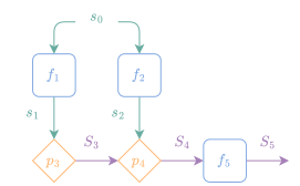
随机程序可以用随机计算图表示，这一概念最初由 [179] 提出。与那项工作不同，我们的论述明确支持两类中间运算：从条件分布中采样，或对函数求值。这些运算既可以产生确定性变量，也可以产生随机变量。A stochastic program can be represented by a stochastic computation graph as originally introduced by [179]. Departing from that work, our exposition explicitly supports two types of intermediate operations: sampling from a conditional distribution or evaluating a function. These operations can produce either deterministic variables or random variables.

函数节点与分布节点Function and distribution nodes

形式上，我们将随机计算图定义为一个有向无环图 $\mathcal{G}=(\mathcal{V},\mathcal{E})$ ，其中 $\mathcal{V}=\mathcal{V}_{f}\cup\mathcal{V}_{p}$ ， $\mathcal{V}_{f}$ 是函数节点集合， $\mathcal{V}_{p}$ 是分布节点集合。与 4.1.3 节中回顾的计算图类似，我们将节点编号为 $\mathcal{V}=\{0,1,\ldots,K\}$ 。节点 $0$ 对应输入 ${\bm{s}}_{0}\in\mathcal{S}_{0}$ ，我们假定它是确定性的；它也是我们希望对其求导的变量。节点 $K$ 对应程序输出 $S_{K}\in\mathcal{S}_{K}$ ，我们假定它是一个随机变量。节点 $k\in\{1,\dots,K\}$ 既可以是函数节点 $k\in\mathcal{V}_{f}$ ，并关联一个函数 $f_{k}$ ，也可以是分布节点 $k\in\mathcal{V}_{p}$ ，并关联一个条件分布 $p_{k}$ 。随机程序至少有一个分布节点，即随机性的来源；否则，它就是一个确定性程序。与计算图一样，边集 $\mathcal{E}$ 用于表示节点之间的依赖关系。我们将节点 $k$ 的父节点记为 ${\operatorname{pa}}(k)$ 。Formally, we define a stochastic computation graph as a directed acyclic graph $\mathcal{G}=(\mathcal{V},\mathcal{E})$ , where $\mathcal{V}=\mathcal{V}_{f}\cup\mathcal{V}_{p}$ , $\mathcal{V}_{f}$ is the set of function nodes and $\mathcal{V}_{p}$ is the set of distribution nodes. Similarly to computation graphs reviewed in Section 4.1.3, we number the nodes as $\mathcal{V}=\{0,1,\ldots,K\}$ . Node $0$ corresponds to the input ${\bm{s}}_{0}\in\mathcal{S}_{0}$ , which we assume to be deterministic. It is the variable with respect to which we wish to differentiate. Node $K$ corresponds to the program output $S_{K}\in\mathcal{S}_{K}$ , which we assume to be a random variable. A node $k\in\{1,\dots,K\}$ can either be a function node $k\in\mathcal{V}_{f}$ with an associated function $f_{k}$ or a distribution node $k\in\mathcal{V}_{p}$ , with associated conditional distribution $p_{k}$ . A stochastic program has at least one distribution node, the source of randomness. Otherwise, it is a deterministic program. As for computation graphs, the set of edges $\mathcal{E}$ is used to represent dependencies between nodes. We denote the parents of node $k$ by ${\operatorname{pa}}(k)$ .

确定性变量与随机变量Deterministic and random variables

我们区分两类中间变量：确定性变量 ${\bm{s}}_{k}$ 与随机变量 $S_{k}$ 。因此，一个分布 $p_{k}$ 或一个函数 $f_{k}$ 都可能接收这两类变量作为条件或输入。于是，将 ${\operatorname{pa}}(k)$ 拆分为 ${\operatorname{pa}}(k)={\operatorname{determ}}(k)\cup{\operatorname{random}}(k)$ 会比较方便，其中我们定义了确定性父节点 ${\operatorname{determ}}(k)\coloneqq\{i_{1},\ldots,i_{p_{k}}\}$ 与随机父节点 ${\operatorname{random}}(k)\coloneqq\{j_{1},\ldots,j_{q_{k}}\}$ 。因此， ${\bm{s}}_{i_{1}},\ldots,{\bm{s}}_{i_{p_{k}}}$ 是节点 $k$ 的确定性父变量， $S_{j_{1}},\ldots,S_{j_{q_{k}}}$ 则是其随机父变量。We distinguish between two types of intermediate variables: deterministic variables ${\bm{s}}_{k}$ and random variables $S_{k}$ . Therefore, a distribution $p_{k}$ or a function $f_{k}$ may receive both types of variables as conditioning or input. It is then convenient to split ${\operatorname{pa}}(k)$ as ${\operatorname{pa}}(k)={\operatorname{determ}}(k)\cup{\operatorname{random}}(k)$ , where we defined the deterministic parents ${\operatorname{determ}}(k)\coloneqq\{i_{1},\ldots,i_{p_{k}}\}$ and the random parents ${\operatorname{random}}(k)\coloneqq\{j_{1},\ldots,j_{q_{k}}\}$ . Therefore, ${\bm{s}}_{i_{1}},\ldots,{\bm{s}}_{i_{p_{k}}}$ are the deterministic parent variables and $S_{j_{1}},\ldots,S_{j_{q_{k}}}$ are the random parent variables, of node $k$ .

执行随机程序Executing a stochastic program

我们假定节点 $0,1,\dots,K$ 处于拓扑序中（若非如此，则需先执行拓扑排序）。给定父变量 ${\bm{s}}_{i_{1}},\ldots,{\bm{s}}_{i_{p_{k}}}$ 与 $S_{j_{1}},\ldots,S_{j_{q_{k}}}$ ，节点 $k\in\{1,\dots,K\}$ 按如下方式产生输出。We assume that nodes $0,1,\dots,K$ are in topological order (if this is not the case, we need to perform a topological sort). Given parent variables ${\bm{s}}_{i_{1}},\ldots,{\bm{s}}_{i_{p_{k}}}$ and $S_{j_{1}},\ldots,S_{j_{q_{k}}}$ , a node $k\in\{1,\dots,K\}$ produces an output as follows.

•

若 $k\in\mathcal{V}_{p}$ （分布节点），则输出为If $k\in\mathcal{V}_{p}$ (distribution node), the output is

	$\displaystyle S_{k}\sim p_{k}(\cdot\mid{\bm{s}}_{{\operatorname{determ}}(k)},S_{{\operatorname{random}}(k)})$
$\displaystyle\iff$	$\displaystyle S_{k}\sim p_{k}(\cdot\mid{\bm{s}}_{i_{1}},\ldots,{\bm{s}}_{i_{p_{k}}},S_{j_{1}},\ldots,S_{j_{q_{k}}})$

注意，从技术上讲， $p_{k}$ 是在给定其父节点的条件下 $S_{k}$ 的分布，而非 $S_{k}$ 的分布。因此，原则上我们应写作 $S_{k}\mid{\bm{s}}_{{\operatorname{determ}}(k)},S_{{\operatorname{random}}(k)}\sim p_{k}(\cdot\mid{\bm{s}}_{{\operatorname{determ}}(k)},S_{{\operatorname{random}}(k)})$ 。为简洁起见，并与函数节点保持对称，我们避免使用这种记号。Note that technically $p_{k}$ is the distribution of $S_{k}$ conditioned on its parents, not the distribution of $S_{k}$ . Therefore, we should in principle write $S_{k}\mid{\bm{s}}_{{\operatorname{determ}}(k)},S_{{\operatorname{random}}(k)}\sim p_{k}(\cdot\mid{\bm{s}}_{{\operatorname{determ}}(k)},S_{{\operatorname{random}}(k)})$ . We avoid this notation for conciseness and for symmetry with function nodes.

与函数节点不同，分布节点可以没有父节点。也就是说，若 $k\in\mathcal{V}_{p}$ ，则 ${\operatorname{pa}}(k)=\emptyset$ 可能成立。无参数的噪声分布就是一个很好的例子。Contrary to a function node, a distribution node can have no parents. That is, if $k\in\mathcal{V}_{p}$ , it is possible that ${\operatorname{pa}}(k)=\emptyset$ . A good example would be a parameter-free noise distribution.

•

若 $k\in\mathcal{V}_{f}$ （函数节点），则输出一般为If $k\in\mathcal{V}_{f}$ (function node), the output is in general

$\displaystyle S_{k}$	$\displaystyle\coloneqq f_{k}({\bm{s}}_{{\operatorname{determ}}(k)},S_{{\operatorname{random}}(k)})$
	$\displaystyle\coloneqq f_{k}({\bm{s}}_{i_{1}},\ldots,{\bm{s}}_{i_{p_{k}}},S_{j_{1}},\ldots,S_{j_{q_{k}}})$

而在特殊情形 $q_{k}=|{\operatorname{random}}(k)|=0$ 下，输出为and in the special case $q_{k}=|{\operatorname{random}}(k)|=0$ , the output is

$\displaystyle{\bm{s}}_{k}$	$\displaystyle\coloneqq f_{k}({\bm{s}}_{{\operatorname{determ}}(k)})$
	$\displaystyle\coloneqq f_{k}({\bm{s}}_{i_{1}},\ldots,{\bm{s}}_{i_{p_{k}}}).$

除非所关联的条件分布 $p_{k}$ 是 delta 分布——即把所有概率质量集中在一个点上——否则分布节点 $k\in\mathcal{V}_{p}$ 的输出必然是一个随机变量 $S_{k}\in\mathcal{S}_{k}$ 。对于函数节点 $k\in\mathcal{V}_{f}$ ，只要 $k$ 的父节点中至少有一个产生随机变量，函数 $f_{k}$ 的输出 $S_{k}\in\mathcal{S}_{k}$ 就是随机变量。反之，若 $k$ 的所有父节点都产生确定性变量，则 $f_{k}$ 的输出是确定性变量 ${\bm{s}}_{k}\in\mathcal{S}_{k}$ 。Unless the associated conditional distribution $p_{k}$ is a delta distribution, that puts all the probability mass on a single point, the output of a distribution node $k\in\mathcal{V}_{p}$ is necessarily a random variable $S_{k}\in\mathcal{S}_{k}$ . For function nodes $k\in\mathcal{V}_{f}$ , the output of the function $f_{k}$ is a random variable $S_{k}\in\mathcal{S}_{k}$ if at least one of the parents of $k$ produces a random variable. Otherwise, if all parents of $k$ produce deterministic variables, the output of $f_{k}$ is a deterministic variable ${\bm{s}}_{k}\in\mathcal{S}_{k}$ .

整个过程总结在算法 1 中。我们强调， $S_{K}=f({\bm{s}}_{0})\in\mathcal{S}_{K}$ 是一个随机变量。因此，随机程序（隐式地）诱导出 $S_{K}$ 上的分布，同时也诱导出中间随机变量 $S_{k}$ 上的分布。执行该随机程序，便可以从该分布中抽取样本。The entire procedure is summarized in Algorithm 1. We emphasize that $S_{K}=f({\bm{s}}_{0})\in\mathcal{S}_{K}$ is a random variable. Therefore, a stochastic program (implicitly) induces a distribution over $S_{K}$ , and also over intermediate random variables $S_{k}$ . Executing the stochastic program allows us to draw samples from that distribution.

算法 1 执行随机程序Algorithm 1 Executing a stochastic program

1: Nodes:

1,\dots,K

in topological order, where node

k

is either a function

f_{k}

or a conditional distribution

p_{k}

2: Input: input

{\bm{s}}_{0}\in\mathcal{S}_{0}

3: for

k\coloneqq 1,\ldots,K

4: Retrieve

{\operatorname{pa}}(k)={\operatorname{determ}}(k)\cup{\operatorname{random}}(k)

5: if

k\in\mathcal{V}_{p}

then

\triangleright

Distribution node

S_{k}\sim p_{k}(\cdot|{\bm{s}}_{{\operatorname{determ}}(k)},S_{{\operatorname{random}}(k)})

7: else if

k\in\mathcal{V}_{f}

then

\triangleright

Function node

8: if

|{\operatorname{random}}(k)|\neq 0

then

S_{k}\coloneqq f_{k}({\bm{s}}_{{\operatorname{determ}}(k)},S_{{\operatorname{random}}(k)})

\triangleright

Output is a R.V.

10: else if

|{\operatorname{random}}(k)|=0

then

11:

{\bm{s}}_{k}\coloneqq f_{k}({\bm{s}}_{{\operatorname{determ}}(k)})

\triangleright

Output is deterministic

12: Output:

f({\bm{s}}_{0})\coloneqq S_{K}\in\mathcal{S}_{K}

特殊情形Special cases

若所有节点都是函数节点，我们就得到计算图，这在 4.1.3 节中已有回顾。若所有节点都是分布节点，我们就得到贝叶斯网络，这在 10.5 节中已有回顾。If all nodes are function nodes, we recover computation graphs, reviewed in Section 4.1.3. If all nodes are distribution nodes, we recover Bayesian networks, reviewed in Section 10.5.

12.5.2 示例Examples

下面给出几个例子，用以说明这一形式化框架。在后续插图中，我们采用下面的图例。We now present several examples that illustrate our formalism. We use the legend below in the following illustrations.

•

例 1（SFE 估计量）：Example 1 (SFE estimator):

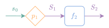
$\displaystyle S_{1}$	$\displaystyle\sim p_{1}(\cdot\mid{\bm{s}}_{0})$
$\displaystyle S_{2}$	$\displaystyle\coloneqq f_{2}(S_{1})$
$\displaystyle E({\bm{s}}_{0})$	$\displaystyle\coloneqq\mathbb{E}[S_{2}]$
$\displaystyle\nabla E({\bm{s}}_{0})$	$\displaystyle=\mathbb{E}_{S_{1}}[f_{2}(S_{1})\nabla_{{\bm{s}}_{0}}\log p_{1}(S_{1}\mid{\bm{s}}_{0})]$

•

例 2（路径估计量）：Example 2 (Pathwise estimator):

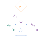
$\displaystyle S_{1}$	$\displaystyle\sim p_{1}$
$\displaystyle S_{2}$	$\displaystyle\coloneqq f_{2}(S_{1},{\bm{s}}_{0})$
$\displaystyle E({\bm{s}}_{0})$	$\displaystyle\coloneqq\mathbb{E}[S_{2}]$
$\displaystyle\nabla E({\bm{s}}_{0})$	$\displaystyle=\mathbb{E}_{S_{1}}\left[\nabla_{{\bm{s}}_{0}}f_{2}(S_{1},{\bm{s}}_{0})\right]$

•

例 3（SFE 估计量 + 链式法则）：Example 3 (SFE estimator + chain rule):

$\displaystyle{\bm{s}}_{1}$	$\displaystyle\coloneqq f_{1}({\bm{s}}_{0})$
$\displaystyle S_{2}$	$\displaystyle\sim p_{2}(\cdot\mid{\bm{s}}_{1})$
$\displaystyle S_{3}$	$\displaystyle\coloneqq f_{3}(S_{2})$
$\displaystyle E({\bm{s}}_{0})$	$\displaystyle\coloneqq\mathbb{E}[S_{3}]$
$\displaystyle\nabla E({\bm{s}}_{0})$	$\displaystyle=\partial f({\bm{s}}_{0})^{*}\mathbb{E}_{S_{2}}[f_{3}(S_{2})\nabla_{{\bm{s}}_{1}}\log p_{2}(S_{2}\mid{\bm{s}}_{1})]$

•

例 4：Example 4:

$\displaystyle{\bm{s}}_{1}$	$\displaystyle\coloneqq f_{1}({\bm{s}}_{0})$
$\displaystyle{\bm{s}}_{2}$	$\displaystyle\coloneqq f_{2}({\bm{s}}_{0})$
$\displaystyle S_{3}$	$\displaystyle\sim p_{3}(\cdot\mid{\bm{s}}_{1})$
$\displaystyle S_{4}$	$\displaystyle\sim p_{4}(\cdot\mid{\bm{s}}_{2},S_{3})$
$\displaystyle S_{5}$	$\displaystyle\coloneqq f_{5}(S_{4})$
$\displaystyle E({\bm{s}}_{0})$	$\displaystyle\coloneqq\mathbb{E}[S_{5}]=\mathbb{E}_{S_{3}}\left[\mathbb{E}_{S_{4}}[f_{5}(S_{4})]\right]$
$\displaystyle\nabla E({\bm{s}}_{0})$	$\displaystyle=\mathbb{E}_{S_{3}}\left[\partial f_{1}({\bm{s}}_{0})^{*}\nabla_{{\bm{s}}_{1}}\log p(S_{3}\mid{\bm{s}}_{1})\mathbb{E}_{S_{4}}[f_{5}(S_{4})]\right]$
	$\displaystyle\quad+\mathbb{E}_{S_{3}}\left[\mathbb{E}_{S_{4}}\left[\partial f_{2}({\bm{s}}_{0})^{*}\nabla_{{\bm{s}}_{2}}\log p_{4}(S_{4}\|{\bm{s}}_{2},S_{3})f_{5}(S_{4})\right]\right]$

可以看到，梯度表达式很快就会变得相当复杂，这也体现了自动微分在随机计算图中的优势。As can be seen, the gradient expressions can quickly become quite complicated, demonstrating the merits of automatic differentiation in stochastic computation graphs.

12.5.3 无偏梯度估计量Unbiased gradient estimators

随机程序的输出是一个随机变量The output of a stochastic program is a random variable

S_{K}\coloneqq f({\bm{s}}_{0}).

它隐式地定义了一个概率分布 $p(\cdot|{\bm{s}}_{0})$ ，使得 $S_{K}\sim p(\cdot|{\bm{s}}_{0})$ 。执行一次随机程序，我们就得到来自 $p(\cdot|{\bm{s}}_{0})$ 的一个独立同分布样本。It implicitly defines a probability distribution $p(\cdot|{\bm{s}}_{0})$ such that $S_{K}\sim p(\cdot|{\bm{s}}_{0})$ . Executing the stochastic program once gives us an i.i.d. sample from $p(\cdot|{\bm{s}}_{0})$ .

由于导数是对确定性变量定义的，我们需要一种方法把随机变量转换为确定性变量。一种做法是考虑期望值（另一种做法是考虑众数）Since derivatives are defined for deterministic variables, we need a way to convert a random variable to a deterministic variable. One way to do so is to consider the expected value (another way would be the mode)

E({\bm{s}}_{0})\coloneqq\mathbb{E}[S_{K}]=\mathbb{E}[f({\bm{s}}_{0})]\in\conv(\mathcal{S}_{K}),

其中期望是对 $S_{K}\sim p(\cdot|{\bm{s}}_{0})$ 取的，等价地，也是对中间随机变量 $S_{k}$ 取的where the expectation is over $S_{K}\sim p(\cdot|{\bm{s}}_{0})$ or equivalently over the intermediate random variables $S_{k}$

S_{k}\sim p_{k}(\cdot|{\bm{s}}_{{\operatorname{determ}}(k)},S_{{\operatorname{random}}(k)}),

对于 $k\in\mathcal{V}_{p}$ （即各个分布节点）。于是我们希望计算 $E({\bm{s}}_{0})$ 的梯度，或者更一般地，计算其雅可比矩阵。for $k\in\mathcal{V}_{p}$ (the distribution nodes). We then wish to compute the gradient or more generally the Jacobian of $E({\bm{s}}_{0})$ .

如果随机计算图中的所有节点都是函数节点，我们可以使用路径梯度估计量（又称重参数化技巧，见 12.4 节）来估计 $E({\bm{s}}_{0})$ 的梯度。这正是文献 [107] 和 [168] 所采用的方法。If all nodes in the stochastic computation graph are function nodes, we can estimate the gradient of $E({\bm{s}}_{0})$ using the pathwise estimator a.k.a. reparametrization trick (Section 12.4). This is the approach taken by [107] and [168].

如果随机计算图中的所有节点都是分布节点，我们可以使用 SFE 估计量（见 12.3 节）。[179] 提出了一种替代损失，对该损失使用自动微分所得的梯度是期望梯度的无偏估计，而这一过程用的正是 SFE 估计量。[68] 将该方法扩展至支持高阶微分。[112] 进一步扩展了该方法，使其支持为每个节点选用不同的估计量，并支持控制变量。If all nodes in the stochastic computation graph are distribution nodes, we can use the SFE estimator (Section 12.3). [179] propose a surrogate loss so that using autodiff on that loss produces an unbiased gradient of the expectation, using the SFE estimator. [68] extend the approach to support high-order differentiation. [112] further extend the approach by supporting different estimators per node, as well as control variates.

将分布节点转换为函数节点及其逆过程Converting distribution nodes into function nodes and vice-versa

我们的形式化框架使用两类节点：带有相应条件分布 $p_{k}$ 的分布节点，以及带有相应函数 $f_{k}$ 的函数节点。通常可以在两类节点之间相互转换。Our formalism uses two types of nodes: distribution nodes with associated conditional distribution $p_{k}$ and function nodes with associated function $f_{k}$ . It is often possible to convert between node types.

将分布节点转换为函数节点，正是 12.4 节所研究的重参数化技巧。我们可以借助位置—尺度变换或逆变换等变换方法来实现。Converting a distribution node into a function node is exactly the reparametrization trick studied in Section 12.4. We can use transformations such as the location-scale transform or the inverse transform.

将函数节点转换为分布节点，则可对前推分布应用 12.4.5 节所研究的变量替换定理来完成。Converting a function node into a distribution node can be done using the change-of-variables theorem, studied in Section 12.4.5, on a pushforward distribution.

由于路径梯度估计量的方差低于 SFE，因此在 $f_{k}$ 函数可用时，它是首选方法。分布节点与函数节点之间的相互转换如图 12.1 所示。Because the pathwise estimator has lower variance than SFE, this is the method of choice when the $f_{k}$ functions are available. The conversion from distribution node to function node and vice-versa is illustrated in Fig. 12.1.

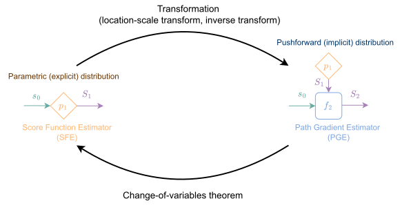
图 12.1：有时可以利用合适的变换，将分布节点转换为函数节点，反之亦然。Figure 12.1: It is sometimes possible to convert a distribution node to a function node and vice-versa using a suitable transformation.

12.5.4 局部期望与全局期望Local vs. global expectations

随机计算图可以视为一个随机过程，即一族随机变量 $S_{k}$ ，以拓扑序中的位置 $k$ 为索引。然而，随机变量与自动微分并不相容。用其期望值替换随机变量，可以看作一种使其与自动微分相容的方式。于是便有两种可能的策略。A stochastic computation graph can be seen as a stochastic process, a collection of random variables $S_{k}$ , indexed by $k$ , the position in the topological order. However, random variables are incompatible with autodiff. Replacing random variables by their expectation can be seen as a way to make them compatible with autodiff. Two strategies are then possible.

如上一节所述，一种策略是考虑最终输出 $S_{K}$ 的期望。该策略对应于全局平滑。它有两个主要优点：i) 我们无需假设 $f_{k+1}$ 在 $\conv(\mathcal{S}_{k})$ 上良定义；ii) 它在程序执行上诱导出一个概率分布。例如，这对于计算程序的方差很有用。程序期望值的梯度可以依据所用节点的类型，通过重参数化技巧或 SFE 来估计。As we saw in the previous section, a strategy is to consider the expectation of the last output $S_{K}$ . This strategy corresponds to a global smoothing. The two major advantages are that i) we do not need to assume that $f_{k+1}$ is well-defined on $\conv(\mathcal{S}_{k})$ and ii) this induces a probability distribution over program executions. This is for instance useful to compute the variance of the program. The gradient of the program’s expected value can be estimated by the reparametrization trick or by the SFE, depending on the type of nodes used.

第二种策略是把中间随机变量 $S_{k}\in\mathcal{S}_{k}$ （其中 $k\in\{1,\dots,K\}$ ）替换为其期望 $\mathbb{E}[S_{k}]\in\conv(\mathcal{S}_{k})$ 。该策略对应于局部平滑。这种做法的潜在缺点在于： $\mathbb{E}[S_{k}]$ 属于 $\conv(\mathcal{S}_{k})$ ，即 $\mathcal{S}_{k}$ 的凸包。因此，以 $\mathbb{E}[S_{k}]$ 为输入的函数 $f_{k+1}$ 必须在 $\conv(\mathcal{S}_{k})$ 上良定义，而实际情况未必总是如此。对控制流而言，另一个缺点来自计算。我们在 5.6 节和 5.7 节已经看到，在条件语句中使用软比较运算符，会在一个二值或分类随机变量上诱导出一个分布，该变量对应着待选的分支。于是，将这一随机变量替换为其期望——即所有分支的凸组合——即可对条件语句做局部平滑。这意味着，除非该分布的支撑集是稀疏的，否则必须对所有分支求值。A second strategy is to replace an intermediate random variable $S_{k}\in\mathcal{S}_{k}$ , for $k\in\{1,\dots,K\}$ , by its expectation $\mathbb{E}[S_{k}]\in\conv(\mathcal{S}_{k})$ . This strategy corresponds to a local smoothing. A potential drawback of this approach is that $\mathbb{E}[S_{k}]$ belongs to $\conv(\mathcal{S}_{k})$ , the convex hull of $\mathcal{S}_{k}$ . Therefore, the function $f_{k+1}$ in which $\mathbb{E}[S_{k}]$ is fed must be well-defined on $\conv(\mathcal{S}_{k})$ , which may not always be the case. In the case of control flows, another disadvantage is computational. We saw in Section 5.6 and Section 5.7 that using a soft comparison operator within a conditional statement induces a distribution on a binary or categorical random variable, corresponding to the branch to be selected. A conditional statement can then be locally smoothed out by replacing the random variable by its expectation i.e., a convex combination of all the branches. This means that, unless the distribution has sparse support, all branches must be evaluated.

12.6 微分方程12.6 Differential equations

12.6.1 参数化微分方程Parameterized differential equations

从残差网络到神经常微分方程From residual networks to neural ODEs

从 ${\bm{s}}_{0}\coloneqq{\bm{x}}$ 出发，4.6 节回顾的残差网络对 $k\in\{1,\dots,K\}$ 进行迭代Starting from ${\bm{s}}_{0}\coloneqq{\bm{x}}$ , residual networks, reviewed in Section 4.6, iterate for $k\in\{1,\dots,K\}$

{\bm{s}}_{k}\coloneqq{\bm{s}}_{k-1}+h_{k}({\bm{s}}_{k-1},{\bm{w}}_{k}).

残差网络可以看作是对离散时间下输入的增量变化做参数化（“残差”之名即由此而来）。A residual network can be seen as parameterizing incremental discrete-time input changes (hence the name “residual”)

{\bm{s}}_{k}-{\bm{s}}_{k-1}=h_{k}({\bm{s}}_{k-1},{\bm{w}}_{k}).

[43] 则提出对连续时间（瞬时）的变化做参数化。他们考虑了输入在连续时间中的演化 ${\bm{s}}(t)$ ：该演化由函数 $h(t,{\bm{s}},{\bm{w}})$ 驱动，而此函数以 ${\bm{w}}$ 为参数，起点为 ${\bm{x}}$ 。形式上，演化 ${\bm{s}}(t)$ 是如下常微分方程（ODE）的解[43] proposed to parameterize continuous-time (instantaneous) changes instead. They considered the evolution ${\bm{s}}(t)$ of the inputs in continuous time driven by a function $h(t,{\bm{s}},{\bm{w}})$ parameterized by ${\bm{w}}$ , starting from ${\bm{x}}$ . Formally, the evolution ${\bm{s}}(t)$ is the solution of the ordinary differential equation (ODE)

$\displaystyle{\bm{s}}(0)$	$\displaystyle={\bm{x}}$
$\displaystyle{\bm{s}}^{\prime}(t)$	$\displaystyle=h(t,{\bm{s}}(t),{\bm{w}})\quad t\in[0,T]$	(12.5)

这里， ${\bm{s}}^{\prime}(t)$ 是 ${\bm{s}}$ 的导数向量，其定义见注 2.2.9； $T$ 表示轨迹的终止时间。于是，这类神经常微分方程 [43] 的输出为 $f({\bm{x}},{\bm{w}})\coloneqq{\bm{s}}(T)$ 。也可以把输出视为某个积分问题的解Here, ${\bm{s}}^{\prime}(t)$ is the vector of derivatives of ${\bm{s}}$ as defined in Remark 2.2.9, and $T$ denotes a final time for the trajectory. The output of such a neural ODE [43] is then $f({\bm{x}},{\bm{w}})\coloneqq{\bm{s}}(T)$ . Alternatively, the output can be seen as the solution of an integration problem

f({\bm{x}},{\bm{w}})={\bm{s}}(T)={\bm{x}}+\int_{0}^{T}h(t,{\bm{s}}(t),{\bm{w}})dt.

(12.6)

像式 12.5 这样的微分方程，其应用远不止神经常微分方程，从物理系统建模到流行病建模 [35] 都有涉及。此外，式 12.5 给出的只是一个常微分方程的例子，受控微分方程或随机微分方程同样可以考虑。Differential equations like Eq. 12.5 arise in many contexts beyond neural ODEs, ranging from modeling physical systems to pandemics [35]. Moreover, the differential equation presented in Eq. 12.5 is just an example of an ordinary differential equation, while controlled differential equations or stochastic differential equations can also be considered.

解的存在性Existence of a solution

首要的问题是 ${\bm{s}}(t)$ 是否良定义。幸运的是，在较弱的条件下答案就是肯定的，如下面回顾的 Picard-Lindelöf 定理所示 [39，定理 16]。First and foremost, the question is whether ${\bm{s}}(t)$ is well-defined. Fortunately, the answer is positive under mild conditions, as shown by Picard-Lindelöf’s theorem recalled below [39, Theorem 16].

定理 12.6.1（ODE 解的存在性与唯一性）。Theorem 12.6.1 (Existence and uniqueness of ODE solutions).

若

h:[0,T]\times\mathcal{S}\rightarrow\mathcal{S}

关于其第一个变量连续、关于第二个变量Lipschitz 连续，则存在唯一可微映射

{\bm{s}}:[0,T]\rightarrow\mathcal{S}

满足If

h:[0,T]\times\mathcal{S}\rightarrow\mathcal{S}

is continuous in its first variable and Lipschitz-continuous in its second variable, then there exists a unique differentiable map

{\bm{s}}:[0,T]\rightarrow\mathcal{S}

satisfying

\displaystyle{\bm{s}}(0)

\displaystyle={\bm{s}}_{0}

\displaystyle{\bm{s}}^{\prime}(t)

\displaystyle=h(t,{\bm{s}}(t))\quad t\in[0,T],

其中

{\bm{s}}_{0}\in\mathcal{S}

为给定值。for some given

{\bm{s}}_{0}\in\mathcal{S}

对于与时间无关的线性函数 $h(t,{\bm{s}})={\bm{A}}{\bm{s}}$ ，式 12.6 中的积分可由下式以闭式形式算出For time-independent linear functions $h(t,{\bm{s}})={\bm{A}}{\bm{s}}$ , the integral in Eq. 12.6 can be computed in closed form as

{\bm{s}}_{t}=\exp(t{\bm{A}})({\bm{s}}_{0}),

其中 $\exp({\bm{A}})$ 为矩阵指数。因此，输出 ${\bm{s}}(T)$ 可以表示为参数的简单函数（此处即为 ${\bm{A}}$ ）。然而在一般情况下，我们并不具备此类解析解，于是正如第 11 章求解优化问题那样，只能诉诸某些迭代算法。where $\exp({\bm{A}})$ is the matrix exponential. Hence, the output ${\bm{s}}(T)$ can be expressed as a simple function of the parameters ( ${\bm{A}}$ in this case). However, generally, we do not have access to such analytical solutions, and, just as for solving optimization problems in Chapter 11, we need to resort to some iterative algorithms.

积分方法Integration methods

要数值求解 ODE，可采用积分方法，其目标是构造序列 ${\bm{s}}_{k}$ ，使之在时刻 $t_{k}$ 处逼近解 ${\bm{s}}(t)$ 。最简单的积分方法是显式欧拉法，它把时刻 $t_{k-1}$ 与 $t_{k}$ 之间的解近似为To numerically solve an ODE, we can use integration methods, whose goal is to build a sequence ${\bm{s}}_{k}$ that approximates the solution ${\bm{s}}(t)$ at times $t_{k}$ . The simplest integration method is the explicit Euler method, which approximates the solutions between times $t_{k-1}$ and $t_{k}$ as

$\displaystyle{\bm{s}}(t_{k-1})-{\bm{s}}(t_{k})$	$\displaystyle=\int_{t_{k-1}}^{t_{k}}h(t,{\bm{s}}(t),{\bm{w}})dt$
	$\displaystyle\approx\delta_{k}h(t_{k-1},{\bm{s}}(t_{k-1}),{\bm{w}}),$

对于一个时间步for a time-step

\delta_{k}\coloneqq t_{k}-t_{k-1}.

由此得到的积分方案是：从 ${\bm{s}}_{0}={\bm{x}}$ 出发，对 $k\in\{1,\ldots,K\}$ 依次计算The resulting integration scheme consists in computing starting from ${\bm{s}}_{0}={\bm{x}}$ , for $k\in\{1,\ldots,K\}$ ,

{\bm{s}}_{k}\coloneqq{\bm{s}}_{k-1}+\delta_{k}h(t_{k-1},{\bm{s}}_{k-1},{\bm{w}}).

把 $\delta_{k}h(t_{k-1},{\bm{s}}_{k-1},{\bm{w}})$ 与 $h_{k}({\bm{s}}_{k-1},{\bm{w}}_{k})$ 视作等同，便可看出残差网络本质上就是用显式欧拉法对神经常微分方程所做的离散化；更确切地说，是对非自治神经常微分方程所做的离散化，参见例如 [52]。Assimilating $\delta_{k}h(t_{k-1},{\bm{s}}_{k-1},{\bm{w}})$ with $h_{k}({\bm{s}}_{k-1},{\bm{w}}_{k})$ , we find that residual networks are essentially the discretization of a neural ODE by an explicit Euler method; more precisely, a non-autonomous neural ODE, see e.g. [52].

欧拉前向法只是众多积分方法中的一种。略举数例，尚有隐式欧拉法、半隐式方法、Runge-Kutta 方法、线性多步方法等。详细综述可参见例如 [74]。积分方法的质量以其一致性和稳定性来衡量 [74]。这两个概念自然会影响 ODE 求值与求导技术的发展。下文对其作简要概述。Euler’s forward method is only one integration method among many. To cite a few, there are implicit Euler methods, semi-implicit methods, Runge-Kutta methods, linear multistep methods, etc. See, e.g., [74] for a detailed review. The quality of an integration method is measured by its consistency and its stability [74]. These concepts naturally influence the development of evaluation and differentiation techniques for ODEs. We briefly summarize them below.

给定固定时间区间 $\delta_{k}=\delta$ 与 $K=\lceil T/\delta\rceil$ 个点，若当 $\delta\rightarrow 0$ 时 $\|{\bm{s}}_{k}-{\bm{s}}(k\delta)\|=O(\delta^{k})$ ，从而 $k\rightarrow+\infty$ ，则称该积分方法是 $k$ 阶一致的。阶数 $k$ 越高，欲在所考虑的各点上达到近似误差 $\varepsilon$ 所需的点便越少。 $\|{\bm{s}}_{k}-{\bm{s}}(k\delta)\|=O(\delta^{k})$ 这一项令人联想到有限差分（第 7 章）中的误差，称为截断误差。Given a fixed time interval $\delta_{k}=\delta$ and $K=\lceil T/\delta\rceil$ points, an integration method is consistent of order $k$ if $\|{\bm{s}}_{k}-{\bm{s}}(k\delta)\|=O(\delta^{k})$ as $\delta\rightarrow 0$ and therefore $k\rightarrow+\infty$ . The higher the order $k$ , the fewer points we need to reach an approximation error $\varepsilon$ on the points considered. The term $\|{\bm{s}}_{k}-{\bm{s}}(k\delta)\|=O(\delta^{k})$ is reminiscent of the error encountered in finite differences (Chapter 7) and is called the truncation error.

方法的（绝对）稳定性，定义为满足如下条件的时间步长所构成的集合：该积分方法能够对某个 $\lambda\in\mathbb{C}$ 积分 $s^{\prime}(t)=\lambda s(t)$ ，且当 $t\rightarrow+\infty$ 时不发散。The (absolute) stability of a method is defined by the set of time-steps such that the integration method can integrate $s^{\prime}(t)=\lambda s(t)$ for some $\lambda\in\mathbb{C}$ without blowing up as $t\rightarrow+\infty$ .

12.6.2 连续伴随法Continuous adjoint method

由于不同的参数 ${\bm{w}}$ 会在式 12.5 中诱导出与 $h(t,{\bm{s}},{\bm{w}})$ 相关联的不同轨迹，我们或许希望通过最小化某个准则来选取其中一条轨迹。例如，可以考虑通过最小化轨迹终点处的损失 $L$ 来选取 ${\bm{w}}\in\mathcal{W}$ ，Since different parameters ${\bm{w}}$ induce different trajectories associated with $h(t,{\bm{s}},{\bm{w}})$ in Eq. 12.5, we may want to select one of these trajectories by minimizing some criterion. For example, we may consider selecting ${\bm{w}}\in\mathcal{W}$ by minimizing a loss $L$ on the final point of the trajectory,

\min_{{\bm{w}}\in\mathcal{W}}L(f({\bm{x}},{\bm{w}}),{\bm{y}}),

(12.7)

其中where

f({\bm{x}},{\bm{w}})\coloneqq{\bm{s}}(T)={\bm{x}}+\int_{0}^{T}h(t,{\bm{s}}(t),{\bm{w}})dt.

为了求解这类问题，需要通过 ODE 解的 VJP 来获得 $L$ 与 $f$ 复合后的梯度。借助下文介绍的连续时间伴随法 [160]，这些 VJP 实际上可被刻画为某个 ODE 本身的解，其证明推迟到 12.6.6 节。To solve such problems, we need to access gradients of $L$ composed with $f$ through VJPs of the solution of the ODE. The VJPs can actually be characterized as solutions of an ODE themselves thanks to the continuous time adjoint method [160], presented below, and whose proof is postponed to Section 12.6.6.

命题 12.6.2（连续时间伴随法）。Proposition 12.6.2 (Continuous-time adjoint method).

考虑函数

h:[0,T]\times\mathcal{S}\times\mathcal{W}\rightarrow\mathcal{S}

，它关于第一个变量连续，关于第二个变量Lipschitz 连续且连续可微。假设对任意

t,{\bm{s}},{\bm{w}}

，

\partial_{3}h(t,{\bm{s}},{\bm{w}})

均存在，且同样关于第一个变量连续、关于第二个变量Lipschitz 连续。记

{\bm{s}}:[0,T]\rightarrow\mathcal{S}

为如下 ODE 的解Consider a function

h:[0,T]\times\mathcal{S}\times\mathcal{W}\rightarrow\mathcal{S}

, continuous in its first variable, Lipschitz-continuous and continuously differentiable in its second variable. Assume that

\partial_{3}h(t,{\bm{s}},{\bm{w}})

exists for any

t,{\bm{s}},{\bm{w}}

, and is also continuous in its first variable, Lipschitz-continuous in its second variable. Denote

{\bm{s}}:[0,T]\rightarrow\mathcal{S}

the solution of the ODE

\displaystyle{\bm{s}}(0)

\displaystyle={\bm{x}}

\displaystyle{\bm{s}}^{\prime}(t)

\displaystyle=h(t,{\bm{s}}(t),{\bm{w}})\quad t\in[0,T],

并记

f({\bm{x}},{\bm{w}})={\bm{s}}(T)

为该 ODE 在时刻

T

的最终状态。and

f({\bm{x}},{\bm{w}})={\bm{s}}(T)

the final state of the ODE at time

T

. 于是，函数

f

可微；对于输出方向

{\bm{u}}\in\mathcal{S}

，其沿

{\bm{u}}

的 VJP 由下式给出Then, the function

f

is differentiable, and for an output direction

{\bm{u}}\in\mathcal{S}

, its VJP along

{\bm{u}}

is given by

\partial f({\bm{x}},{\bm{w}})^{*}{\bm{u}}=({\bm{r}}(0),{\bm{g}})

对于for

{\bm{g}}=\int_{0}^{T}\partial_{3}h(t,{\bm{s}}(t),{\bm{w}})^{*}{\bm{r}}(t)dt

以及对满足伴随（反向）ODE 的

{\bm{r}}

and for

{\bm{r}}

solving the adjoint (backward) ODE

\displaystyle{\bm{r}}^{\prime}(t)

\displaystyle=-\partial_{2}h(t,{\bm{s}}(t),{\bm{w}})^{*}{\bm{r}}(t)

\displaystyle{\bm{r}}(T)

\displaystyle={\bm{u}}.

特别地，当

L:\mathcal{S}\rightarrow\mathbb{R}

为可微损失时，梯度

\nabla(L\circ f)({\bm{x}},{\bm{w}})

可通过以

{\bm{r}}(T)=\nabla L({\bm{s}}(T))

求解伴随 ODE 得到。In particular, the gradient

\nabla(L\circ f)({\bm{x}},{\bm{w}})

for

L:\mathcal{S}\rightarrow\mathbb{R}

a differentiable loss is obtained by solving the adjoint ODE with

{\bm{r}}(T)=\nabla L({\bm{s}}(T))

例 12.6.3（通过 ODE 的解拟合数据）。Example 12.6.3 (Fitting data through the solution of an ODE).

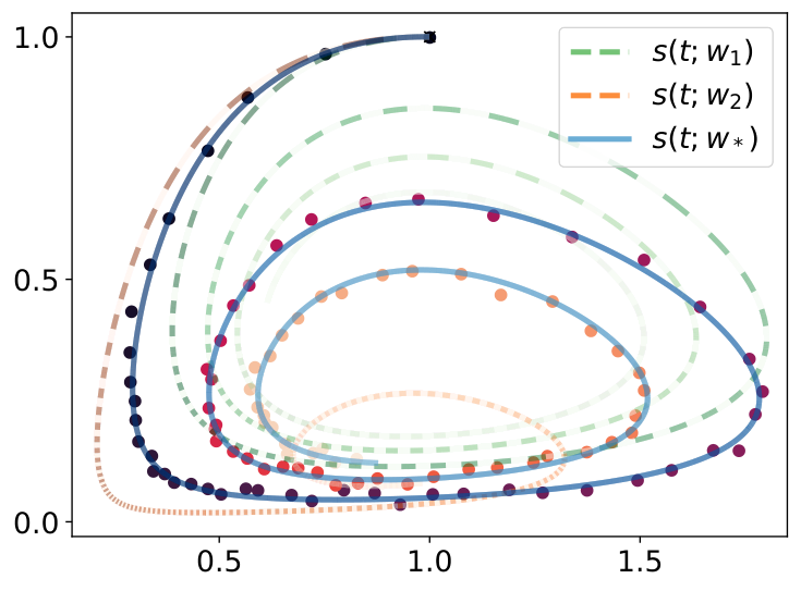
作为一个说明性示例，我们可以考虑优化 ODE 的参数以拟合若干数据点。也就是说，我们可以寻找修改后的 Lotka Volterra ODE 的连续时间解

{\bm{z}}(t;{\bm{w}})

As an illustrative example, we can consider optimizing the parameters of an ODE to fit some data points. Namely, we may seek a continuous time solution

{\bm{z}}(t;{\bm{w}})

of a modified Lotka Volterra ODE

{\bm{z}}^{\prime}(t;{\bm{w}})=\begin{pmatrix}\alpha z_{1}(t;{\bm{w}})-\beta z_{1}(t;{\bm{w}})z_{2}(t;{\bm{w}})\\ -\gamma z_{2}(t;{\bm{w}})+\delta z_{1}(t;{\bm{w}})z_{2}(t;{\bm{w}})\end{pmatrix}+{\bm{c}},

对于

{\bm{w}}=(\alpha,\beta,\gamma,\delta,{\bm{c}})

，使其拟合某些观测

{\bm{z}}_{1},\ldots,{\bm{z}}_{T}

。于是，优化问题由下式构成for

{\bm{w}}=(\alpha,\beta,\gamma,\delta,{\bm{c}})

, that fits some observations

{\bm{z}}_{1},\ldots,{\bm{z}}_{T}

. The optimization problem then consists of

\min_{{\bm{w}}}\sum_{j=1}^{T}\|{\bm{z}}(t_{j};{\bm{w}})-{\bm{z}}_{j}\|^{2},

并要求对 ODE 的解

{\bm{z}}(\cdot;{\bm{w}})

关于其候选参数

{\bm{w}}

进行反向传播。图 12.2 以不同的候选参数说明了这样一个问题。and requires backpropagating through the solution

{\bm{z}}(\cdot;{\bm{w}})

of the ODE w.r.t. its candidate parameters

{\bm{w}}

. Fig. 12.2 illustrates such a problem with varying candidate parameters.

Refer to caption — 图 12.2：寻找 ODE 的最优参数以拟合某些观测数据。图中点表示在规则时间点上观测到的动力系统轨迹（此处时间由渐变色表示，颜色越浅，时间越大）。每条线表示由某些超参数 ${\bm{w}}$ 确定的 ODE 的解。目标是找到 ODE 的超参数，使其解能够拟合这些数据点。绿色和橙色线条未能做到这一点，而蓝色线条则拟合了数据。为了计算这样的参数 ${\bm{w}}$ ，需要沿着 ODE 的解进行反向传播。Figure 12.2: Finding the optimal parameters of an ODE to fit some observed data. The dots represent the trajectories of a dynamical system observed at regular times (time is represented here by a gradient color, the lighter the color, the larger the time). Each line represents the solution of an ODE given by some hyperparameters ${\bm{w}}$ . The objective is to find the hyperparameters of the ODE such that its solution fits the data points. Green and orange lines fail to do so while the blue line fits the data. To compute such parameters ${\bm{w}}$ , we need to backpropagate through the solution of the ODE.

12.6.3 通过连续伴随法计算梯度Gradients via the continuous adjoint method

命题 12.6.2 给出了梯度的形式化定义。然而，正如计算映射 $f({\bm{x}},{\bm{w}})$ 本身一样，计算其 VJP 或 $L\circ f$ 的梯度也需要求解一个积分问题。注意，命题 12.6.2 中对 ${\bm{r}}(t)$ 的积分还需要 ${\bm{s}}(t)$ 的取值。因此，需要同时积分 ${\bm{r}}(t)$ 与 ${\bm{s}}(t)$ 。这种方法通常被称为先优化后离散：首先在连续时间下表述梯度（即“优化部分”），然后对所得的 ODE 进行离散化。Proposition 12.6.2 gives a formal definition of the gradient. However, just as computing the mapping $f({\bm{x}},{\bm{w}})$ itself, computing its VJP or the gradient of $L\circ f$ requires solving an integration problem. Note that the integration of ${\bm{r}}(t)$ in Proposition 12.6.2 requires also values of ${\bm{s}}(t)$ . Therefore, we need to integrate both ${\bm{r}}(t)$ and ${\bm{s}}(t)$ . Such an approach is generally referred to as optimize-then-discretize because we first formulate the gradient in continuous time (the “optimize part”) and then discretize the resulting ODE.

简单的离散化方案Simple discretization scheme

第一种方法是定义一个反向离散化方案，使其能够在时间上反向近似 ${\bm{s}}(t)$ 。具体而言，通过定义 ${\bm{\sigma}}(t)={\bm{s}}(T-t),{\bm{\rho}}(t)={\bm{r}}(T-t)$ 与 ${\bm{\gamma}}(t)=\int_{t}^{T}\partial_{3}h(\tau,{\bm{s}}(\tau),{\bm{w}})^{*}{\bm{r}}(\tau)d\tau$ ， $L\circ f$ 的导数由 $({\bm{\rho}}(T),{\bm{\gamma}}(T))$ 给出。函数 ${\bm{\sigma}},{\bm{\rho}},{\bm{\gamma}}$ 是标准 ODE 的解A first approach consists in defining a backward discretization scheme that can approximate ${\bm{s}}(t)$ backward in time. Namely, by defining ${\bm{\sigma}}(t)={\bm{s}}(T-t),{\bm{\rho}}(t)={\bm{r}}(T-t)$ , and ${\bm{\gamma}}(t)=\int_{t}^{T}\partial_{3}h(\tau,{\bm{s}}(\tau),{\bm{w}})^{*}{\bm{r}}(\tau)d\tau$ , the derivative of $L\circ f$ is given by $({\bm{\rho}}(T),{\bm{\gamma}}(T))$ . The functions ${\bm{\sigma}},{\bm{\rho}},{\bm{\gamma}}$ are solutions of a standard ODE

$\displaystyle{\bm{\sigma}}(0)$	$\displaystyle={\bm{s}}(T),\hskip 30.0pt{\bm{\sigma}}^{\prime}(t)=-h(T-t,{\bm{\sigma}}(t),{\bm{w}}),$
$\displaystyle{\bm{\rho}}(0)$	$\displaystyle=\nabla L({\bm{s}}(T)),\hskip 6.0pt{\bm{\rho}}^{\prime}(t)=\partial_{2}h(T-t,{\bm{\sigma}}(t),{\bm{w}})^{*}{\bm{\rho}}(t),$
$\displaystyle{\bm{\gamma}}(0)$	$\displaystyle=0,\hskip 48.0pt{\bm{\gamma}}^{\prime}(t)=\partial_{3}h(T-t,{\bm{\sigma}}(t),{\bm{w}})^{*}{\bm{\rho}}(t).$

上述 ODE 随后可用任意积分方法求解。但请注意，这需要先通过某种积分方法计算 ${\bm{s}}(T)$ 与 $\nabla L({\bm{s}}(T))$ 。使用显式欧拉法求解前向与后向 ODE 从而计算梯度的整体过程总结于算法 2。The above ODE can then be solved by any integration method. Note, however, that it requires first computing ${\bm{s}}(T)$ and $\nabla L({\bm{s}}(T))$ by an integration method. The overall computation of the gradient using an explicit Euler method to solve forward and backward ODEs is summarized in Algorithm 2.

算法 2 通过采用显式欧拉离散化的连续伴随法计算梯度Algorithm 2 Gradient computation via continuous adjoint method with Euler explicit discretization

1: Functions:

h:[0,T]\times\mathcal{S}\times\mathcal{W}\rightarrow\mathbb{R}

L:\mathcal{S}\rightarrow\mathbb{R}

2: Inputs: input

{\bm{x}}

, parameters

{\bm{w}}

, number of discretization steps

K

3: Set discretization step

\delta=T/K

, denote

h_{k}({\bm{s}},{\bm{w}})=h(k\delta,{\bm{s}},{\bm{w}})

4: Set

{\bm{s}}_{0}\coloneqq{\bm{x}}

5: for

k\coloneqq 1,\ldots,K

\triangleright

Forward discretization

6: Compute

{\bm{s}}_{k}\coloneqq{\bm{s}}_{k-1}+\delta h_{k-1}({\bm{s}}_{k-1},{\bm{w}})

7: Compute

{\bm{u}}\coloneqq\nabla L({\bm{s}}_{K})

8: Initialize

{\bm{r}}_{K}\coloneqq{\bm{u}}

\hat{\bm{s}}_{K}={\bm{s}}_{K}

{\bm{g}}_{K}={\mathbf{0}}

9: for

k\coloneqq K,\ldots,1

\triangleright

Backward discretization

10: Compute

\hat{\bm{s}}_{k-1}\coloneqq\hat{\bm{s}}_{k}-\delta h_{k}(\hat{\bm{s}}_{k},{\bm{w}})

11: Compute

{\bm{r}}_{k-1}\coloneqq{\bm{r}}_{k}+\delta\partial_{2}h_{k}(\hat{\bm{s}}_{k},{\bm{w}})^{*}{\bm{r}}_{k}

12: Compute

{\bm{g}}_{k-1}\coloneqq{\bm{g}}_{k}+\delta\partial_{3}h_{k}(\hat{\bm{s}}_{k},{\bm{w}})^{*}{\bm{r}}_{k}

13: Output:

({\bm{r}}_{0},{\bm{g}}_{0})\approx\nabla(L\circ f)({\bm{x}},{\bm{w}})

算法 2 从形式上看，与权重共享的残差神经网络的反向模式自动微分如出一辙。但有一个显著区别：中间计算 ${\bm{s}}_{k}$ 并不保存在内存中，而是沿反向 ODE 计算新的变量 $\hat{\bm{s}}_{k}$ 。人们或许以为，改用连续时间后，反向模式自动微分中遇到的内存问题便已解决。遗憾的是，这是以数值稳定性为代价的。在算法 2 中，我们要借助离散化方案，通过 $\hat{\bm{s}}_{k}$ 在时间上反向重新计算中间状态，因此会累积一些截断误差。Algorithm 2 naturally looks like the reverse mode of autodiff for a residual neural network with shared weights. A striking difference is that the intermediate computations ${\bm{s}}_{k}$ are not kept in memory and, instead, new variables $\hat{\bm{s}}_{k}$ are computed along the backward ODE. One may believe that by switching to continuous time, we solved the memory issues encountered in reverse-mode autodiff. Unfortunately, this comes at the cost of numerical stability. As we use a discretization scheme to recompute the intermediate states backward in time through $\hat{\bm{s}}_{k}$ in Algorithm 2, we accumulate some truncation errors.

要理解这里的问题，不妨对同一组参数反复应用算法 2，但每次用 $\hat{\bm{s}}_{0}$ 代替 ${\bm{s}}_{0}={\bm{x}}$ 。在连续情形下， ${\bm{\sigma}}(T)={\bm{s}}(0)$ 。然而经过离散化后， $\hat{\bm{s}}_{0}\approx{\bm{\sigma}}(T)$ 与 ${\bm{s}}_{0}$ 并不相等。因此，若以 ${\bm{s}}_{0}=\hat{\bm{s}}_{0}$ 应用算法 2，即使连续时间下本应自然得到相同结果，实际输出也不会相同。图 12.3 展示了这一现象，直观地说明了算法 2 为何会在梯度估计中引入噪声。To understand the issue here, consider applying Algorithm 2 repeatedly on the same parameters but using $\hat{\bm{s}}_{0}$ instead of ${\bm{s}}_{0}={\bm{x}}$ each time. In the continuous realm, ${\bm{\sigma}}(T)={\bm{s}}(0)$ . But after discretization, $\hat{\bm{s}}_{0}\approx{\bm{\sigma}}(T)$ does not match ${\bm{s}}_{0}$ . Therefore, by applying Algorithm 2 with ${\bm{s}}_{0}=\hat{\bm{s}}_{0}$ , we would not get the same output even if in continuous time we naturally should have. This phenomenon is illustrated in Fig. 12.3. It intuitively shows why Algorithm 2 induces some noise in the estimation of the gradient.

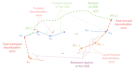
图 12.3：使用连续伴随法时的前向与后向离散化。Figure 12.3: Forward and backward discretizations when using the continuous adjoint method.

多重打靶方案Multiple shooting scheme

另一种思路是将前向 ODE 与后向 ODE 联合积分，即求解一个带边界值的 ODEAn alternative approach consists in integrating both the forward and backward ODEs jointly. Namely, we may solve an ODE with boundary values

$\displaystyle{\bm{s}}^{\prime}(t)$	$\displaystyle=h(t,{\bm{s}}(t),{\bm{w}}),\quad{\bm{s}}(0)={\bm{x}},$
$\displaystyle{\bm{r}}^{\prime}(t)$	$\displaystyle=-\partial_{2}h(t,{\bm{s}}(t),{\bm{w}})^{*}{\bm{r}}(t),\quad{\bm{r}}(T)=\nabla L({\bm{s}}(T))$
$\displaystyle{\bm{g}}^{\prime}(t)$	$\displaystyle=-\partial_{3}h(t,{\bm{s}}(t),{\bm{w}})^{*}{\bm{r}}(t),\quad{\bm{g}}(T)=0,$

可采用多重打靶法或配点法 [187] 求解。该方法仍需先近似 $\nabla L({\bm{s}}(T))$ 。by means of a multiple shooting method or a collocation method [187]. This approach still requires $\nabla L({\bm{s}}(T))$ to be approximated first.

12.6.4 基于离散化的反向模式计算梯度Gradients via reverse-mode on discretization

还有一种更简单的做法：用某种数值方法（例如欧拉前向离散化方案）将式 12.7 中的目标函数离散化，再以其离散版本取而代之。也就是说，我们要求解A simpler approach consists in replacing the objective in Eq. 12.7 by its version discretized using some numerical method, such as an Euler forward discretization scheme. That is, we seek to solve

\min_{{\bm{w}}\in\mathcal{W}}\quad L({\bm{s}}_{K})\quad\text{where}\quad{\bm{s}}_{k}={\bm{s}}_{k-1}+\delta h(k\delta,{\bm{s}}_{k-1},{\bm{w}}) \ k\in\{1,\ldots,K\},

其中 ${\bm{s}}_{0}={\mathbf{0}}$ 与 $\delta$ 为某个离散化步长。目标函数的梯度可通过自动微分计算。这种方法通常称为先离散化、后优化。乍看之下，它可能带来极高的内存需求。确实，为获得 ODE 的准确解，数值积分方法可能要求 $K$ 非常大。由于反向模式自动微分的朴素实现所需内存随 $K$ 线性增长，以先离散化、后优化方法计算梯度可能令人望而却步。不过，如 8.5 节所述，借助检查点技术可轻松摊销内存需求；另见 [77]。with ${\bm{s}}_{0}={\mathbf{0}}$ and $\delta$ some discretization step. Gradients of the objective can be computed by automatic differentiation. That approach is often referred to as discretize-then-optimize. At first glance, this approach may suffer from very high memory requirements. Indeed, to get an accurate solution of the ODE, a numerical integration method may require $K$ to be very large. Since a naive implementation of reverse-mode automatic differentiation has a memory that scales linearly with $K$ , computing the gradient by a discretize-then-optimize method could be prohibitive. However, the memory requirements may easily be amortized using checkpointing, as explained in Section 8.5; see also [77].

至于先优化后离散方法，我们在前向离散化过程中仍会累积一些截断误差。在反向模式下计算梯度时也会出现这种离散化误差。先离散化、后优化方法可以视为在计算某个替代目标函数的梯度。对该目标函数而言，梯度是正确的，也是良定义的。然而，它们未必与真实 ODE 表述的梯度相符。As for the optimize-then-discretize method, we still accumulate some truncation errors in the forward discretization process. This discretization error occurs when computing the gradient in reverse-mode too. The discretize-then-optimize method can be seen as computing gradients of a surrogate objective. For that objective, the gradients are correct and well-defined. However, they may not match the gradients of the true ODE formulation.

为比较先离散化、后优化与先优化后离散两种方法，[77] 在一个其解可解析计算的 ODE 上比较了二者性能，其做法是取 $h$ 为关于 ${\bm{s}}$ 的线性函数。作者观察到，先离散化、后优化通常优于先优化后离散。实际上，若采用可逆的求导方案，则可以找到一种折中。To compare the discretize-then-optimize and optimize-then-discretize approaches, [77] compared their performance on an ODE whose solution can be computed analytically by selecting $h$ to be linear in ${\bm{s}}$ . The authors observed that discretize-then-optimize generally outperformed optimize-then-discretize. A middle ground can actually be found by using reversible differentiation schemes.

12.6.5 可逆离散化方案Reversible discretization schemes

我们对先优化后离散方法与先离散化、后优化方法的阐述采用了简单的欧拉显式离散化方案。然而，对这两种方法，我们本可以改用其他离散化方案，例如可逆离散化方案。Our exposition of the optimize-then-discretize or discretize-then-optimize approaches used a simple Euler explicit discretization scheme. However, for both approaches, we could have used other discretization schemes instead, such as reversible discretization schemes.

可逆离散化方案是一种这样的离散化方案：其离散化步的逆具有闭式公式。形式上，离散化方法 $\mathcal{M}$ 通过在区间 $[0,T]$ 上对 $k\in(1,\dots,K)$ 计算下式，构造 ODE ${\bm{s}}^{\prime}(t)=h(t,{\bm{s}}(t))$ 的解的近似 $({\bm{s}}_{k})_{k=1}^{K}$ ：A reversible discretization scheme is a discretization scheme such that we have access to a closed-form formula for the inverse of its discretization step. Formally, a discretization method $\mathcal{M}$ builds an approximation $({\bm{s}}_{k})_{k=1}^{K}$ of the solution of an ODE ${\bm{s}}^{\prime}(t)=h(t,{\bm{s}}(t))$ on an interval $[0,T]$ by computing for $k\in(1,\dots,K)$

\displaystyle t_{k},{\bm{s}}_{k},{\bm{c}}_{k}=\mathcal{M}(t_{k-1},{\bm{s}}_{k-1},{\bm{c}}_{k-1};h,\delta),

(12.8)

其中 $\delta>0$ 是某个固定的离散化步， $t_{k}$ 是时间步（通常为 $t_{k}=t_{k-1}+\delta$ ）， ${\bm{s}}_{k}$ 是 ${\bm{s}}(t_{k})$ 的近似， ${\bm{c}}_{k}$ 是离散化方法用于构造迭代值的一些附加上下文变量。显式欧拉法没有上下文，但正如优化方法可能更新某些内部状态一样，离散化方法也可以更新某些上下文变量。式 12.8 中的离散化方案是前向离散化方案，因为我们采用了正的离散化步。取负的离散化步，便得到相应的后向离散化方案，对 $k\in(K,\dots,1)$ ，where $\delta>0$ is some fixed discretization step, $t_{k}$ is the time step (typically $t_{k}=t_{k-1}+\delta$ ), ${\bm{s}}_{k}$ is the approximation of ${\bm{s}}(t_{k})$ , and ${\bm{c}}_{k}$ is some additional context variable used by the discretization method to build the iterates. An explicit Euler method does not have a context, but just as an optimization method may update some internal states, a discretization method can update some context variable. The discretization scheme in Eq. 12.8 is a forward discretization scheme as we took a positive discretization step. By taking a negative discretization step, we obtain the corresponding backward discretization scheme, for $k\in(K,\dots,1)$ ,

\displaystyle t_{k-1},{\bm{s}}_{k-1},{\bm{c}}_{k-1}=\mathcal{M}(t_{k},{\bm{s}}_{k},{\bm{c}}_{k};h,-\delta).

若我们能借助 $\mathcal{M}^{-1}$ 由其输出重新计算该离散化步的输入，则该离散化方法是可逆的，A discretization method is reversible if we have access to $\mathcal{M}^{-1}$ to recompute the inputs of the discretization step from its outputs,

t_{k-1},{\bm{s}}_{k-1},{\bm{c}}_{k}=\mathcal{M}^{-1}(t_{k},{\bm{s}}_{k},{\bm{c}}_{k};h,\delta).

若后向离散化方案恰好是前向离散化方案的逆，则称该可逆离散化方法是对称的，即A reversible discretization method is symmetric if the backward discretization scheme is exactly the inverse of the forward discretization scheme, i.e.,

\displaystyle\mathcal{M}(t_{k},{\bm{s}}_{k},{\bm{c}}_{k};h,-\delta)=\mathcal{M}^{-1}(t_{k},{\bm{s}}_{k},{\bm{c}}_{k};h,\delta).

显式欧拉法显然不是对称的，并且先验地不可逆，除非我们能对 ${\bm{y}}_{k-1}$ 解出方程 ${\bm{y}}_{k}={\bm{y}}_{k-1}+\delta f({\bm{y}}_{k-1})$ 。The explicit Euler method is clearly not symmetric and a priori not reversible, unless we can solve for ${\bm{y}}_{k-1}$ , the equation ${\bm{y}}_{k}={\bm{y}}_{k-1}+\delta f({\bm{y}}_{k-1})$ .

Leapfrog 方法Leapfrog method

另一方面，（异步）leapfrog 方法 [216, 142] 是对称可逆离散化方法的一个例子。对于常数离散化步 $\delta$ ，给定 $t_{k-1},{\bm{s}}_{k-1},{\bm{c}}_{k-1}$ 和函数 $h$ ，它计算The (asynchronous) leapfrog method [216, 142] on the other hand is an example of symmetric reversible discretization method. For a constant discretization step $\delta$ , given $t_{k-1},{\bm{s}}_{k-1},{\bm{c}}_{k-1}$ and a function $h$ , it computes

$\displaystyle\bar{t}_{k-1}$	$\displaystyle\coloneqq t_{k-1}+\frac{\delta}{2}$
$\displaystyle\bar{\bm{s}}_{k-1}$	$\displaystyle\coloneqq{\bm{s}}_{k-1}+\frac{\delta}{2}{\bm{c}}_{k-1}$
$\displaystyle\bar{\bm{c}}_{k-1}$	$\displaystyle\coloneqq h(\bar{t}_{k-1},\bar{\bm{s}}_{k-1})$
$\displaystyle t_{k}$	$\displaystyle\coloneqq\bar{t}_{k-1}+\frac{\delta}{2}$
$\displaystyle{\bm{s}}_{k}$	$\displaystyle\coloneqq\bar{\bm{s}}_{k-1}+\frac{\delta}{2}\bar{\bm{c}}_{k-1}$
$\displaystyle{\bm{c}}_{k}$	$\displaystyle\coloneqq 2\bar{\bm{c}}_{k-1}-{\bm{c}}_{k-1}$
$\displaystyle\mathcal{M}(t_{k-1},{\bm{s}}_{k-1},{\bm{c}}_{k-1};h,\delta)$	$\displaystyle\coloneqq(t_{k},{\bm{s}}_{k},{\bm{c}}_{k}).\hskip 60.0pt$

可以验证，我们确实有 $\mathcal{M}(t_{k},{\bm{s}}_{k},{\bm{c}}_{k};h,-\delta)=(t_{k-1},{\bm{s}}_{k},{\bm{c}}_{k})$ 。One can verify that we indeed have $\mathcal{M}(t_{k},{\bm{s}}_{k},{\bm{c}}_{k};h,-\delta)=(t_{k-1},{\bm{s}}_{k},{\bm{c}}_{k})$ .

通过在先优化后离散方法中使用可逆对称离散化方案，我们确保在后向离散化过程结束时，能够精确恢复原始输入。因此，通过反复执行前向与后向离散化方案，我们总能得到相同的梯度，而显式欧拉方案则并非如此。By using a reversible symmetric discretization scheme in the optimize-then-discretize approach, we ensure that, at the end of the backward discretization pass, we recover exactly the original input. Therefore, by repeating forward and backward discretization schemes we always get the same gradient, which was not the case for an Euler explicit scheme.

通过在“先离散化、后优化”方法中使用可逆离散化方案，我们解决了反向模式自动微分的存储问题。正如 8.6 节所述，我们可以在反向传播过程中重新计算中间值，而不必将其存储起来。By using a reversible discretization scheme in the discretize-then-optimize method, we address the memory issues of reverse mode autodiff. As explained in Section 8.6, we can recompute intermediate values during the backward pass rather than storing them.

动量残差神经网络Momentum residual networks

在 leapfrog 方法中，额外变量 ${\bm{c}}_{k}$ 实际上可以解释为某个系统的速度，而该系统的加速度由给定函数驱动，即 ${\bm{s}}^{\prime\prime}(t)=h(t,{\bm{s}}(t),{\bm{w}})$ 。这一解释为通常的神经常微分方程范式提供了替代思路。例如，动量神经网络 [175] 可视为二阶常微分方程的离散化，而这类方程天然适合采用内存占用低的可逆求导方案。In the leapfrog method, the additional variables ${\bm{c}}_{k}$ may actually be interpreted as velocities of a system whose acceleration is driven by the given function, that is, ${\bm{s}}^{\prime\prime}(t)=h(t,{\bm{s}}(t),{\bm{w}})$ . Such an interpretation suggests alternatives to the usual neural ODE paradigm. For instance, momentum neural networks [175], can be interpreted as the discretization of a second-order ordinary differential equation, which is naturally amenable to reversible differentiation schemes with a low memory footprint.

12.6.6 连续伴随法的证明Proof of the continuous adjoint method

下文记 ${\bm{s}}(t,{\bm{x}},{\bm{w}})$ 为给定输入 ${\bm{x}}$ 与参数 ${\bm{w}}$ 时，常微分方程在时刻 $t$ 的解。这里我们聚焦于 VJP 的表述。该证明依赖于 ${\bm{s}}(t,{\bm{x}},{\bm{w}})$ 的偏导数存在性；对此我们不予讨论，读者可参阅例如 [160]，以了解在给定假设下对此类事实的完整证明。In the following, we denote ${\bm{s}}(t,{\bm{x}},{\bm{w}})$ the solution of the ODE at time $t$ given the input ${\bm{x}}$ and the parameters ${\bm{w}}$ . We focus here on the formulation of the VJP. The proof relies on the existence of partial derivatives of ${\bm{s}}(t,{\bm{x}},{\bm{w}})$ , which we do not cover here and refer to, e.g., [160] for a complete proof of such facts given the assumptions.

我们借助常微分方程约束引入伴随变量，这一次将其写成连续可微函数 ${\bm{r}}$ 的形式。对任意这样的函数 ${\bm{r}}$ ，有We use the ODE constraint to introduce adjoint variables, this time in the form of a continuously differentiable function ${\bm{r}}$ . For any such function ${\bm{r}}$ , we have

$\displaystyle\langle f({\bm{x}},{\bm{w}}),{\bm{u}}\rangle$	$\displaystyle=\langle{\bm{s}}(T,{\bm{x}},{\bm{w}}),{\bm{u}}\rangle$
	$\displaystyle\quad+\int_{0}^{T}\langle{\bm{r}}(t),h(t,{\bm{s}}(t,{\bm{x}},{\bm{w}}),{\bm{w}})-\partial_{t}{\bm{s}}(t,{\bm{x}},{\bm{w}})\rangle dt,$

其中采用了诸如 $\partial_{t}{\bm{s}}(t,{\bm{x}},{\bm{w}})=\partial_{1}{\bm{s}}(t,{\bm{x}},{\bm{w}})$ 的莱布尼茨记号。于是 VJP 可分解为using Leibniz notations such as $\partial_{t}{\bm{s}}(t,{\bm{x}},{\bm{w}})=\partial_{1}{\bm{s}}(t,{\bm{x}},{\bm{w}})$ . The VJPs then decompose as

	$\displaystyle\partial_{\bm{w}}f({\bm{x}},{\bm{w}})^{*}[{\bm{u}}]$
	$\displaystyle=\partial_{\bm{w}}{\bm{s}}(T,{\bm{x}},{\bm{w}})^{*}{\bm{u}}$
	$\displaystyle\quad+\int_{0}^{T}(\partial_{\bm{w}}{\bm{s}}(t,{\bm{x}},{\bm{w}})^{}\partial_{\bm{s}}h(t,{\bm{s}}(t,{\bm{x}},{\bm{w}}),{\bm{w}})^{}-\partial_{{\bm{w}}t}^{2}{\bm{s}}(t,{\bm{x}},{\bm{w}})^{*}){\bm{r}}(t)dt$
	$\displaystyle\quad+\int_{0}^{T}\partial_{\bm{w}}h(t,{\bm{s}}(t,{\bm{x}},{\bm{w}}),{\bm{w}})^{*}{\bm{r}}(t)dt,$
	$\displaystyle\partial_{\bm{x}}f({\bm{x}},{\bm{w}})^{*}[{\bm{u}}]$
	$\displaystyle=\partial_{\bm{x}}{\bm{s}}(T,{\bm{x}},{\bm{w}})^{*}{\bm{u}}$
	$\displaystyle\quad+\int_{0}^{T}(\partial_{\bm{x}}{\bm{s}}(t,{\bm{x}},{\bm{w}})^{}\partial_{\bm{s}}h(t,{\bm{s}}(t,{\bm{x}},{\bm{w}}),{\bm{w}})^{}-\partial_{{\bm{x}}t}^{2}{\bm{s}}(t,{\bm{x}},{\bm{w}})^{*}){\bm{r}}(t)dt$

此处的二阶导数项 $\partial_{{\bm{w}}t}^{2}{\bm{s}}(t,{\bm{x}},{\bm{w}})^{*}{\bm{r}},\partial_{{\bm{x}}t}^{2}{\bm{s}}(t,{\bm{x}},{\bm{w}})^{*}{\bm{r}}$ 对应于 $\langle{\bm{s}}(t,{\bm{x}},{\bm{w}}),{\bm{r}}\rangle$ 的二阶导数。由于 Hessian 矩阵是对称的（即命题 2.4.6 所给出的 Schwarz 定理），我们可以交换 $t$ 与 ${\bm{w}}$ 或 ${\bm{x}}$ 中的求导次序。随后，为仅以 ${\bm{s}}$ 的一阶导数表示梯度，我们使用分部积分，例如可得Here the second derivative terms $\partial_{{\bm{w}}t}^{2}{\bm{s}}(t,{\bm{x}},{\bm{w}})^{*}{\bm{r}},\partial_{{\bm{x}}t}^{2}{\bm{s}}(t,{\bm{x}},{\bm{w}})^{*}{\bm{r}}$ correspond to second derivatives of $\langle{\bm{s}}(t,{\bm{x}},{\bm{w}}),{\bm{r}}\rangle$ . Since the Hessian is symmetric (Schwarz’s theorem presented in Proposition 2.4.6), we can swap the derivatives in $t$ and ${\bm{w}}$ or ${\bm{x}}$ . Then, to express the gradient uniquely in terms of first derivatives of ${\bm{s}}$ , we use an integration by parts to have for example

$\displaystyle\int_{0}^{T}\partial_{{\bm{w}}t}^{2}{\bm{s}}(t,{\bm{x}},{\bm{w}})^{*}{\bm{r}}(t)dt$	$\displaystyle=\int_{0}^{T}\partial_{t{\bm{w}}}^{2}{\bm{s}}(t,{\bm{x}},{\bm{w}})^{*}{\bm{r}}(t)dt$
	$\displaystyle=(\partial_{{\bm{w}}}{\bm{s}}(T,{\bm{x}},{\bm{w}})^{}{\bm{r}}(T)-\partial_{{\bm{w}}}{\bm{s}}(0,{\bm{x}},{\bm{w}})^{}{\bm{r}}(0))$
	$\displaystyle\quad-\int_{0}^{T}\partial_{{\bm{w}}}{\bm{s}}(t,{\bm{x}},{\bm{w}})^{*}\partial_{t}{\bm{r}}(t)dt.$

由于 ${\bm{s}}(0)={\bm{x}}$ ，故有 $\partial_{{\bm{w}}}{\bm{s}}(0,{\bm{x}},{\bm{w}})^{*}{\bm{r}}(0)=0$ 。于是关于 ${\bm{w}}$ 的 VJP 可写作Since ${\bm{s}}(0)={\bm{x}}$ , we have $\partial_{{\bm{w}}}{\bm{s}}(0,{\bm{x}},{\bm{w}})^{*}{\bm{r}}(0)=0$ . The VJP w.r.t. ${\bm{w}}$ can then be written as

	$\displaystyle\partial_{\bm{w}}f({\bm{x}},{\bm{w}})^{*}[{\bm{u}}]$
	$\displaystyle=\partial_{\bm{w}}{\bm{s}}(T,{\bm{x}},{\bm{w}})^{*}[{\bm{u}}-{\bm{r}}(T)]$
	$\displaystyle\quad+\int_{0}^{T}\partial_{\bm{w}}{\bm{s}}(t,{\bm{x}},{\bm{w}})^{}[\partial_{\bm{s}}h(t,{\bm{s}}(t,{\bm{x}},{\bm{w}}),{\bm{w}})^{}{\bm{r}}(t)+\partial_{t}{\bm{r}}(t)]dt$
	$\displaystyle\quad+\int_{0}^{T}\partial_{\bm{w}}h(t,{\bm{s}}(t,{\bm{x}},{\bm{w}}),{\bm{w}})^{*}{\bm{r}}(t)dt.$

通过选取 ${\bm{r}}(t)$ 使其满足伴随 ODEBy choosing ${\bm{r}}(t)$ to satisfy the adjoint ODE

\partial_{t}{\bm{r}}(t)=-\partial_{\bm{s}}h(t,{\bm{s}}(t,{\bm{x}},{\bm{w}}),{\bm{w}})^{*}{\bm{r}}(t),\quad{\bm{r}}(T)={\bm{u}},

VJP 的表达式便简化为the expression of the VJP simplifies as

\partial_{\bm{w}}f({\bm{x}},{\bm{w}})^{*}[{\bm{u}}]=\int_{0}^{T}\partial_{\bm{w}}h(t,{\bm{s}}(t,{\bm{x}},{\bm{w}}),{\bm{w}})^{*}{\bm{r}}(t)dt.

对于关于 ${\bm{x}}$ 的 VJP，可同理处理。利用分部积分，此时可得 $\partial_{{\bm{x}}}{\bm{s}}(0,{\bm{x}},{\bm{w}})^{*}{\bm{r}}(0)={\bm{r}}(0)$ ，因为 ${\bm{s}}(0)={\bm{x}}$ 。选取满足伴随 ODE 的同一曲线 ${\bm{r}}(t)$ ，便得到For the VJP w.r.t. ${\bm{x}}$ , we can proceed similarly. Using an integration by parts, we have, this time, $\partial_{{\bm{x}}}{\bm{s}}(0,{\bm{x}},{\bm{w}})^{*}{\bm{r}}(0)={\bm{r}}(0)$ since ${\bm{s}}(0)={\bm{x}}$ . Choosing the same curve ${\bm{r}}(t)$ satisfying the adjoint ODE we get

\partial_{\bm{x}}f({\bm{x}},{\bm{w}})^{*}[{\bm{u}}]={\bm{r}}(0).

作为反向 ODE 的解，曲线 ${\bm{r}}$ 的存在性可由 Picard-Lindelöf 定理并结合相关假设直接推出。The existence of a curve ${\bm{r}}$ solution of the backward ODE can easily be shown from Picard Lindelöf’s theorem and the assumptions.

12.7 小结12.7 Summary

•

我们研究了如何对积分求导，重点关注期望以及微分方程的解。We studied how to differentiate integrals, with a focus on expectations and solutions of a differential equation.
•

对期望进行求导，我们研究了两种主要方法：得分函数估计量（SFE，又称 REINFORCE）与路径梯度估计量（PGE，又称重参数化技巧）。For differentiating through expectations, we studied two main methods: the score function estimator (SFE, a.k.a. REINFORCE) and the path gradient estimator (PGE, a.k.a. reparametrization trick).
•

当分布易于采样、且其对数 PDF 可显式写出时，SFE 较为适用。它虽为无偏估计量，但众所周知方差较大。The SFE is suitable when it is easy to sample from the distribution and its log-PDF is explicitly available. It is an unbiased estimator, but is known to suffer from high variance.
•

PGE 则适用于前推分布，也就是通过一个变换或一连串变换隐式定义的分布。只要把随机性的来源（如噪声）注入这些变换，便很容易从这类分布中采样；而只要能够交换积分与求导的次序，就能便捷地得到其期望梯度的无偏、低方差估计量。The PGE is suitable for pushforward distributions, distributions that are implicitly defined through a transformation, or a sequence of them. These distributions can be easily sampled from, by injecting a source of randomness (such as noise) through the transformations. An unbiased, low-variance estimator of the gradient of their expectation is easily obtained, provided that we can interchange integration and differentiation.
•

若分布是显式的，有时借助位置—尺度变换或逆变换，便可将其化为隐式分布。If we have an explicit distribution, we can sometimes convert it to an implicit distribution, thanks to the location-scale transformation or the inverse transformation.
•

反之，若分布是隐式的，则可借助变量替换定理将其化为显式分布。不过，该公式需要计算逆雅可比矩阵的行列式，通常计算代价高昂；归一化流则从设计上采用可逆变换，使逆雅可比矩阵的计算变得廉价。Conversely, if we have an implicit distribution, we can convert it to an explicit distribution using the change-of-variables theorem. However, this formula requires computing the determinant of an inverse Jacobian, and is computationally expensive in general. Normalizing flows use invertible transformations so that the inverse Jacobian is cheap to compute, by design.
•

在随机计算图中，每个节点都可以混合使用显式分布与隐式分布。Stochastic computation graphs can use a mix of explicit and implicit distributions at each node.
•

对微分方程的解进行求导，可考虑两种途径。For differentiating through the solution of a differential equation, two approaches can be considered.
•

借助连续伴随法，可将梯度表示为某个微分方程的解，再对梯度所满足的微分方程按时间反向离散化，这便是先优化后离散的途径。We can express the gradient as the solution of a differential equation thanks to the continuous adjoint method. We may then discretize backwards in time the differential equation that the gradient satisfies. This is the optimize-then-discretize approach.
•

也可以先对问题离散化，使梯度能够直接通过在离散化步骤上应用反向模式自动微分求得，这便是先离散化、后优化的途径。先优化后离散的途径没有内存开销，但前向与后向离散化过程之间的不一致往往引发数值误差；先离散化、后优化的途径不会产生这种不一致，但可能带来高昂的内存开销。We can also first discretize the problem in such a way that the gradient can simply be computed by reverse mode auto-diff, applied on the discretization steps. This is the discretize-then-optimize approach. The optimize-then-discretize approach has no memory cost, but discrepancies between the forward and backward discretization passes often lead to numerical errors. The discretize-then-optimize approach introduces no such discrepancies but may come at a large memory cost.
•

可逆离散化方案能够按时间反向重新计算中间的离散化步骤，从而绕开内存开销。Reversible discretization schemes can circumvent the memory cost, as they enable the recomputation of intermediate discretization steps backwards in time.

第 12 章 通过积分求导Chapter 12 Differentiating through integration

12.1 积分号下求导12.1 Differentiation under the integral sign

12.2 通过期望求导12.2 Differentiating through expectations

12.2.1 与参数无关的分布Parameter-independent distributions

12.2.2 依赖于参数的分布Parameter-dependent distributions

连续情形Continuous case

离散情形Discrete case

12.2.3 在期望损失函数中的应用Application to expected loss functions

12.2.4 在实验设计中的应用Application to experimental design

12.3 得分函数估计量与 REINFORCE12.3 Score function estimators, REINFORCE

12.3.1 标量值函数Scalar-valued functions

命题 12.3.1（标量值函数的 SFE）。Proposition 12.3.1 (SFE for scalar-valued functions).

证明 12.3.2。Proof 12.3.2.

例 12.3.3（语言模型中的 SFE）。Example 12.3.3 (SFE with a language model).

例 12.3.4（Gibbs 分布中的 SFE）。Example 12.3.4 (SFE with a Gibbs distribution).

同时对分布与函数求导Differentiating through both the distribution and the function

通过联合分布求导Differentiating through joint distributions

12.3.2 方差缩减Variance reduction

偏差与方差Bias and variance

基线Baseline

REINFORCE 留一法（RLOO）REINFORCE leave-one-out (RLOO)

控制变量Control variates

12.3.3 向量值函数Vector-valued functions

命题 12.3.5（向量值函数的 SFE）。Proposition 12.3.5 (SFE for vector-valued functions).

证明 12.3.6。Proof 12.3.6.

同时对分布与函数求导Differentiating through both the distribution and the function

12.3.4 二阶导数Second derivatives

命题 12.3.7（Hessian 矩阵的 SFE）。Proposition 12.3.7 (SFE for the Hessian).

与 Bartlett 恒等式的联系Link with the Bartlett identities

12.3.5 适配自动微分的实现Autodiff-friendly implementation

12.4 路径梯度估计量与重参数化技巧12.4 Path gradient estimators, reparametrization trick

12.4.1 位置—尺度变换Location-scale transforms

命题 12.4.1（位置—尺度族分布的 CDF 与 PDF）。Proposition 12.4.1 (CDF and PDF of location-scale family distributions).

证明 12.4.2。Proof 12.4.2.

12.4.2 可微变换Differentiable transforms

命题 12.4.3（路径梯度估计量）。Proposition 12.4.3 (Path gradient estimator).

例 12.4.4（统计学中的一些可微变换）。Example 12.4.4 (Some differentiable transforms in statistics).

12.4.3 逆变换Inverse transforms

命题 12.4.5（逆变换采样）。Proposition 12.4.5 (Inverse transform sampling).

证明 12.4.6。Proof 12.4.6.

例 12.4.7（分位数函数的例子）。Example 12.4.7 (Examples of quantile functions).

12.4.4 前推算子Pushforward operators

前推分布Pushforward distributions

定义 12.4.8（前推分布）。Definition 12.4.8 (Pushforward distribution).

前推测度Pushforward measures

定义 12.4.9（前推算子与前推测度）。Definition 12.4.9 (Pushforward operator and measure).

12.4.5 变量替换定理Change-of-variables theorem

命题 12.4.10（前推分布的 PDF）。Proposition 12.4.10 (PDF of the pushforward distribution).

12.5 随机程序12.5 Stochastic programs

12.5.1 随机计算图Stochastic computation graphs

函数节点与分布节点Function and distribution nodes

确定性变量与随机变量Deterministic and random variables

执行随机程序Executing a stochastic program

特殊情形Special cases

12.5.2 示例Examples

12.5.3 无偏梯度估计量Unbiased gradient estimators

将分布节点转换为函数节点及其逆过程Converting distribution nodes into function nodes and vice-versa

12.5.4 局部期望与全局期望Local vs. global expectations

12.6 微分方程12.6 Differential equations

12.6.1 参数化微分方程Parameterized differential equations

从残差网络到神经常微分方程From residual networks to neural ODEs

解的存在性Existence of a solution

定理 12.6.1（ODE 解的存在性与唯一性）。Theorem 12.6.1 (Existence and uniqueness of ODE solutions).

积分方法Integration methods

12.6.2 连续伴随法Continuous adjoint method

命题 12.6.2（连续时间伴随法）。Proposition 12.6.2 (Continuous-time adjoint method).

例 12.6.3（通过 ODE 的解拟合数据）。Example 12.6.3 (Fitting data through the solution of an ODE).

12.6.3 通过连续伴随法计算梯度Gradients via the continuous adjoint method

简单的离散化方案Simple discretization scheme

多重打靶方案Multiple shooting scheme

12.6.4 基于离散化的反向模式计算梯度Gradients via reverse-mode on discretization

12.6.5 可逆离散化方案Reversible discretization schemes

Leapfrog 方法Leapfrog method

动量残差神经网络Momentum residual networks

12.6.6 连续伴随法的证明Proof of the continuous adjoint method

12.7 小结12.7 Summary

第 12 章通过积分求导Chapter 12 Differentiating through integration