第 9 章 二阶自动微分Chapter 9 Second-order automatic differentiation

HVP 可以通过四种不同的方式计算。An HVP can be computed in four different ways.

1. 1.

   反向之上的反向：Hessian 矩阵可以看作梯度的转置雅可比矩阵，因此 HVP 可以计算为梯度的 VJP，Reverse on reverse: The Hessian can be seen as the transposed Jacobian of the gradient, hence the HVP can be computed as the VJP of the gradient,

   $$\nabla^{2}f({\bm{w}})[{\bm{v}}]=\partial(\nabla f)({\bm{w}})^{*}[{\bm{v}}].$$

2. 2.

   反向之上的前向：由于Hessian 矩阵是对称的（见命题 2.4.6），它也可以看作梯度的雅可比矩阵，因此 HVP 可以计算为梯度的 JVP，Forward on reverse: Owing to its symmetry (see Proposition 2.4.6), the Hessian can also be seen as the Jacobian of the gradient, hence the HVP can be computed as the JVP of the gradient,

   $$\nabla^{2}f({\bm{w}})[{\bm{v}}]=\partial(\nabla f)({\bm{w}})[{\bm{v}}].$$

3. 3.

   反向之上的前向：回顾对于任意函数 $g\colon\mathcal{E}\to\mathcal{E}$，VJP 可以等价地定义为沿输出方向 ${\bm{v}}\in\mathcal{E}$ 的梯度，即Reverse on forward: Recall that for any function $g\colon\mathcal{E}\to\mathcal{E}$, the VJP can equivalently be defined as the gradient along an output direction ${\bm{v}}\in\mathcal{E}$, that is,

   $$\partial g({\bm{w}})^{*}[{\bm{v}}]=\nabla\langle g,{\bm{v}}\rangle({\bm{w}}),$$

   其中沿用简写 $\langle g,{\bm{v}}\rangle({\bm{w}})\coloneqq\langle{\bm{v}},g({\bm{w}})\rangle$，于是 $\langle g,{\bm{v}}\rangle$ 是 ${\bm{w}}$ 的函数。因此在本例中，我们可以将“反向之上的反向”方法改写为where we recall the shorthand $\langle g,{\bm{v}}\rangle({\bm{w}})\coloneqq\langle{\bm{v}},g({\bm{w}})\rangle$, so that $\langle g,{\bm{v}}\rangle$ is a function of ${\bm{w}}$. In our case, we can therefore rewrite the reverse-on-reverse approach as

   $$\partial(\nabla f)({\bm{w}})^{*}[{\bm{v}}]=\nabla\langle\nabla f,{\bm{v}}\rangle({\bm{w}}).$$

   我们知道 $\langle\nabla f,{\bm{v}}\rangle({\bm{w}})=\langle\nabla f({\bm{w}}),{\bm{v}}\rangle=\partial f({\bm{w}})[{\bm{v}}]$ 是 $f$ 在 ${\bm{w}}$ 处沿 ${\bm{v}}$ 的 JVP。因此，我们也可以将 HVP 计算为 $f$ 在 ${\bm{w}}$ 处沿 ${\bm{v}}$ 的 JVP 的梯度，We know that $\langle\nabla f,{\bm{v}}\rangle({\bm{w}})=\langle\nabla f({\bm{w}}),{\bm{v}}\rangle=\partial f({\bm{w}})[{\bm{v}}]$ is the JVP of $f$ at ${\bm{w}}$ along ${\bm{v}}$. Therefore, we can also compute the HVP as the gradient of the JVP of $f$ at ${\bm{w}}$ along ${\bm{v}}$,

   $$\nabla^{2}f({\bm{w}})[{\bm{v}}]=\nabla(\partial f(\cdot)[{\bm{v}}])({\bm{w}}),$$

   其中采用记号 $(\partial f(\cdot)[{\bm{v}}])({\bm{w}})\coloneqq\partial f({\bm{w}})[{\bm{v}}]$，以强调它是 ${\bm{w}}$ 的函数。where we use the notation $(\partial f(\cdot)[{\bm{v}}])({\bm{w}})\coloneqq\partial f({\bm{w}})[{\bm{v}}]$ to insist on the fact that it is a function of ${\bm{w}}$.

4. 4.

   前向之上的前向：最后，我们可以使用定义 2.4.7 中把 HVP 定义为沿 ${\bm{v}}$ 以及各标准方向的二阶偏导数向量这一点。也就是说，假设 $\mathcal{E}=\mathbb{R}^{P}$，我们可以计算 JVP 的 JVP 共 $P$ 次：Forward on forward: Finally, we can use the definition of the HVP in Definition 2.4.7 as a vector of second partial derivatives along ${\bm{v}}$ and each canonical direction. That is, assuming $\mathcal{E}=\mathbb{R}^{P}$, we can compute the JVP of the JVP $P$ times:

   $$\nabla^{2}f({\bm{w}})[{\bm{v}}]=(\partial^{2}f({\bm{w}})[{\bm{v}},{\bm{e}}_{i}])_{i=1}^{P}.$$

计算 HVP 的四种不同方法汇总于表 9.1。The four different ways of computing the HVP are summarized in Table 9.1.

为直观了解这四种方法的计算复杂度与内存复杂度，我们沿用 8.1 节的做法，考虑一个函数链 $f\coloneqq f_{K}\circ\dots\circ f_{1}$。为简化分析，我们假设对 $k\in\{1,\dots,K-1\}$，有 $f_{k}\colon\mathbb{R}^{P}\to\mathbb{R}^{P}$，且 $f_{K}\colon\mathbb{R}^{P}\to\mathbb{R}$。To get a sense of the computational and memory complexity of the four approaches, we consider a chain of functions $f\coloneqq f_{K}\circ\dots\circ f_{1}$ as done in Section 8.1. To simplify our analysis, we assume $f_{k}\colon\mathbb{R}^{P}\to\mathbb{R}^{P}$ for $k\in\{1,\dots,K-1\}$ and $f_{K}\colon\mathbb{R}^{P}\to\mathbb{R}$.

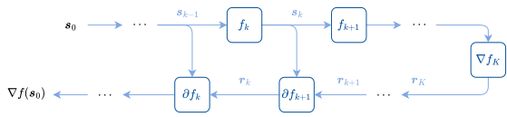
反向模式的计算图如图 9.1 所示。$f=f_{K}\circ\dots\circ f_{1}$ 可以用一条简单的链表示，但 $\nabla f$ 的计算图不再是一条链，而是一个 DAG。这是因为在 $\partial f_{k}({\bm{s}}_{k-1})^{*}[{\bm{r}}_{k}]$ 的计算中，${\bm{s}}_{k-1}$ 与 ${\bm{r}}_{k}$ 都依赖于 ${\bm{s}}_{0}$。The computation graph of the reverse mode is illustrated in Fig. 9.1. While $f=f_{K}\circ\dots\circ f_{1}$ would be represented by a simple chain, the computational graph of $\nabla f$ is no longer a chain: it is a DAG. This is due to the computations of $\partial f_{k}({\bm{s}}_{k-1})^{*}[{\bm{r}}_{k}]$, where both ${\bm{s}}_{k-1}$ and ${\bm{r}}_{k}$ depend on ${\bm{s}}_{0}$.

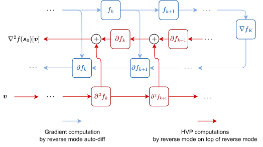
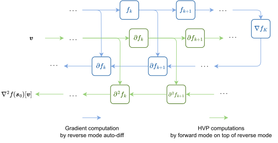
图 9.2 与图 9.3 分别展示了反向之上的反向、反向之上的前向的计算图。在反向模式之上再施加反向模式时，每个扇入运算 ${\bm{s}}_{k-1},{\bm{r}}_{k}\mapsto\partial f_{k}({\bm{s}}_{k-1})^{*}[{\bm{r}}_{k}]$ 处，$\nabla f$ 上的反向模式都会分岔为两条路径，随后由一次求和合并。而在反向模式之上叠加前向模式时，计算流只是沿着 $\nabla f$ 的流程推进。We illustrate the computation graphs of reverse-on-reverse and forward-on-reverse in Fig. 9.2 and Fig. 9.3 respectively. By applying reverse mode on reverse mode, at each fan-in operation ${\bm{s}}_{k-1},{\bm{r}}_{k}\mapsto\partial f_{k}({\bm{s}}_{k-1})^{*}[{\bm{r}}_{k}]$, the reverse mode on $\nabla f$ branches out into two paths that are later merged by a sum. By applying forward mode on top of reverse mode, the flow of computations simply follows that of $\nabla f$.

据此，仿照表 8.1 的计算，可得如下结果。我们假设每个 $\partial f_{k}({\bm{s}}_{k-1})$ 都是稠密线性算子，因而其应用代价与矩阵—向量乘积相同。至于内存复杂度，我们考虑每个运算的输入都会被保存下来，以便在反向传播中计算所需的导数。With this in mind, following a similar calculation as for Table 8.1, we obtain the following results. We assume that each $\partial f_{k}({\bm{s}}_{k-1})$ is a dense linear operator, so that its application has the same cost as a matrix-vector multiplication. For the memory complexity, we consider that the inputs of each operation are saved to compute the required derivatives in the backward passes.

1. 1.

   反向之上的反向：时间为 $O(KP^{2})$，空间为 $O(KP)$。Reverse on reverse: $O(KP^{2})$ time and $O(KP)$ space.

2. 2.

   前向模式叠加于反向模式之上：时间复杂度为 $O(KP^{2})$，空间复杂度为 $O(KP)$。Forward on reverse: $O(KP^{2})$ time and $O(KP)$ space.

3. 3.

   反向模式叠加于前向模式之上：时间复杂度为 $O(KP^{2})$，空间复杂度为 $O(KP)$。Reverse on forward: $O(KP^{2})$ time and $O(KP)$ space.

4. 4.

   前向模式叠加于前向模式之上：对 $P$ 个 JVP，时间复杂度为 $O(KP^{3})$，空间复杂度为 $O(3P)$，其中 ${\bm{e}}_{1},\dots,{\bm{e}}_{P}$。Forward on forward: $O(KP^{3})$ time and $O(3P)$ space for the $P$ JVPs with ${\bm{e}}_{1},\dots,{\bm{e}}_{P}$.

可以看到，对于由函数构成的链，“反向叠加反向”“前向叠加反向”与“反向叠加前向”三者的时间复杂度至多相差若干常数因子，因而大体相当。在反向模式之上再叠加反向模式，需要保存反向传播的信息，即 ${\bm{r}}_{k}$（相应地，保存前向传播的信息，即图 8.1 中的 ${\bm{t}}_{k}$），以便完成最后一次反向传播。若在反向模式之上改用前向模式，便不会产生这项额外开销，内存代价因而略低。此外，反向模式叠加反向模式还会因图 9.2 所示的分支与合并运算而多出若干次求和；反向模式叠加于前向模式之上时同样如此，因为我们无法回避扇入运算（此处其形式为 ${\bm{s}}_{k-1},{\bm{t}}_{k-1}\mapsto\partial f_{k}({\bm{s}}_{k-1})[{\bm{t}}_{k-1}]$）。遗憾的是，“前向叠加前向”的代价高昂得令人望而却步。We see that, for chains of functions, “reverse on reverse”, “forward on reverse” and “reverse on forward” all have similar time complexities up to some constant factors. Using reverse mode on top of reverse mode requires storing the information backpropagated, i.e., the ${\bm{r}}_{k}$ (resp. the information forwarded, i.e., the ${\bm{t}}_{k}$ in Fig. 8.1), to perform the final reverse pass. By using forward mode on top of reverse mode, this additional cost is not incurred, making it slightly less memory expensive. In addition, reverse mode on top of reverse mode induces a few additional summations due to the branching and merge operations depicted in Fig. 9.2. The same holds when using reverse on top of forward as we cannot avoid fan-in operations (this time of the form ${\bm{s}}_{k-1},{\bm{t}}_{k-1}\mapsto\partial f_{k}({\bm{s}}_{k-1})[{\bm{t}}_{k-1}]$). Unfortunately, “forward on forward” is prohibitively expensive.

总之，在计算 HVP 的四种方法中，就计算复杂度与内存复杂度而言，前向叠加反向模式是先验上最可取的一种。不过需要注意的是，高阶导数的计算可以受益于专门设计的自动微分实现，例如泰勒模式自动微分，它们并非只是把前向模式与反向模式简单组合起来。对于一般的函数 $f$，合理的做法是对前三种方法逐一做基准测试，以确定哪一种最适合当前的函数。To summarize, among the four approaches presented to compute HVPs, the forward-on-reverse mode is a priori the most preferable in terms of computational and memory complexities. Note, however, that computations of higher derivatives can benefit from dedicated autodiff implementations such as Taylor mode autodiff, that do not merely compose forward and reverse modes. For general functions $f$, it is reasonable to benchmark the first three methods to determine which method is the best for the function at hand.

函数 $L\colon\mathcal{W}\to\mathbb{R}$ 的 Hessian 矩阵 $\nabla^{2}L({\bm{w}})$ 常被用来构造 $L({\bm{w}})$ 的二次近似，The Hessian matrix $\nabla^{2}L({\bm{w}})$ of a function $L\colon\mathcal{W}\to\mathbb{R}$ is often used to construct a quadratic approximation of $L({\bm{w}})$,

遗憾的是，当 $L$ 非凸时，$\nabla^{2}L({\bm{w}})$ 通常是不定矩阵，也就是说，上述近似是关于 ${\bm{v}}$ 的非凸二次函数。例如，若 $L=\ell\circ f$ 而 $\ell$ 为凸，则当 $f$ 为线性时 $L$ 是凸的；但当 $f$ 非线性时，它通常是非凸的。（广义）Gauss-Newton 矩阵是 Hessian 矩阵的一种有原则的替代，它针对 $L\coloneqq\ell\circ f$ 定义。Unfortunately, when $L$ is nonconvex, $\nabla^{2}L({\bm{w}})$ is typically an indefinite matrix, which means that the above approximation is a nonconvex quadratic w.r.t. ${\bm{v}}$. For instance, if $L=\ell\circ f$ with $\ell$ convex, then $L$ is convex if $f$ is linear, but it is typically nonconvex if $f$ is nonlinear. The (generalized) Gauss-Newton matrix is a principled alternative to the Hessian, which is defined for $L\coloneqq\ell\circ f$.

正如 17.2 节所讨论的，Gauss-Newton 矩阵是 Gauss-Newton 方法的关键要素。其优点之一在于：只要 $\ell$ 为凸，它便是半正定的。As studied in Section 17.2, the Gauss-Newton matrix is a key ingredient of the Gauss-Newton method. An advantage of the Gauss-Newton matrix is its positive semi-definiteness provided that $\ell$ is convex.

这意味着该近似This means that the approximation

是关于 ${\bm{v}}$ 的凸二次函数。is a convex quadratic w.r.t. ${\bm{v}}$.

利用链式法则可知，$L=\ell\circ f$ 的Hessian 矩阵可分解为两项之和（另见命题 9.5.1）。Using the chain rule, we find that the Hessian of $L=\ell\circ f$ decomposes into the sum of two terms (see also Proposition 9.5.1).

因此，Gauss-Newton 算子 $\nabla^{2}_{\mathrm{GN}}(\ell\circ f)$ 可视为 Hessian 矩阵 $\nabla^{2}(\ell\circ f)$ 的一种近似；当 $f$ 为线性时，二者相等。The Gauss-Newton operator $\nabla^{2}_{\mathrm{GN}}(\ell\circ f)$ can therefore be seen as an approximation of the Hessian $\nabla^{2}(\ell\circ f)$, with equality if $f$ is linear.

命题 9.5.1 给出了计算两个函数复合的 Hessian 矩阵的链式法则，但由于交叉项的存在，该公式相对复杂；相比之下，Gauss-Newton 链式法则十分简洁。A chain rule for computing the Hessian of a composition of two functions is presented in Proposition 9.5.1, but the formula is relatively complicated, due to the cross-terms. In contrast, a Gauss-Newton chain rule is straightforward.

与 Hessian 矩阵类似，我们很少需要在内存中具体化完整的 Gauss-Newton 矩阵。事实上，我们可以针对方向 ${\bm{v}}\in\mathcal{W}$ 定义 Gauss-Newton 向量乘积（GNVP），即一个线性映射：As for the Hessian, we rarely need to materialize the full Gauss-Newton matrix in memory. Indeed, we can define the Gauss-Newton vector product (GNVP), a linear map for a direction ${\bm{v}}\in\mathcal{W}$, as

其中 $\nabla^{2}\ell(f({\bm{w}}))[{\bm{u}}]$ 是 $\ell$ 的 HVP，即从 $\mathcal{M}$ 到 $\mathcal{M}$ 的线性映射。GNVP 可以利用 $f$ 的 JVP、$\ell$ 的 HVP 以及 $f$ 的 VJP 来计算。具体化 VJP 需要对 $f$ 进行 $1$ 次前向传播，由此可同时得到值 $f({\bm{w}})$ 和伴随线性映射 ${\bm{u}}\mapsto\partial f({\bm{w}})^{*}[{\bm{u}}]$；求值 VJP 需要对 $f$ 进行 $1$ 次反向传播；求值 JVP 则需要对 $f$ 进行 $1$ 次前向传播。因此，求值 ${\bm{v}}\mapsto\nabla^{2}_{\mathrm{GN}}(\ell\circ f)({\bm{w}})[{\bm{v}}]$ 总共需要对 $f$ 进行 $2$ 次前向传播和 $1$ 次反向传播。where $\nabla^{2}\ell(f({\bm{w}}))[{\bm{u}}]$ is the HVP of $\ell$, a linear map from $\mathcal{M}$ to $\mathcal{M}$. The GNVP can be computed using the JVP of $f$, the HVP of $\ell$ and the VJP of $f$. Instantiating the VJP requires $1$ forward pass through $f$, from which we get both the value $f({\bm{w}})$ and the adjoint linear map ${\bm{u}}\mapsto\partial f({\bm{w}})^{*}[{\bm{u}}]$. Evaluating the VJP requires $1$ backward pass through $f$. Evaluating the JVP requires $1$ forward pass through $f$. In total, evaluating ${\bm{v}}\mapsto\nabla^{2}_{\mathrm{GN}}(\ell\circ f)({\bm{w}})[{\bm{v}}]$ therefore requires $2$ forward passes and $1$ backward pass through $f$.

在本节中，我们假定 $\mathcal{W}\subseteq\mathbb{R}^{P}$ 且 $\mathcal{M}\subseteq\mathbb{R}^{M}$。当 $\ell$ 为凸函数时，Gauss-Newton 矩阵是半正定的，因此可分解为 $\nabla^{2}_{\mathrm{GN}}(\ell\circ f)({\bm{w}})=VV^{\top}$，其中 $V\in\mathbb{R}^{P\times R}$，$R\leq\min\{P,M\}$ 为该矩阵的秩。这一分解实际上可以很方便地由 $\ell$ 的 Hessian 矩阵的因子分解算出。例如，设已知 $\ell$ 的 Hessian 矩阵的特征分解 $\nabla^{2}\ell(f({\bm{w}}))=\sum_{i=1}^{M}\lambda_{i}{\bm{u}}_{i}{\bm{u}}_{i}^{\top}$，其中 ${\bm{u}}_{i}$ 为特征向量，$\lambda_{i}\geq 0$ 为特征值（由半正定性可知这些特征值非负）。于是，Gauss-Newton 矩阵可分解为In this section, we assume $\mathcal{W}\subseteq\mathbb{R}^{P}$ and $\mathcal{M}\subseteq\mathbb{R}^{M}$. When $\ell$ is convex, we know that the Gauss-Newton matrix is positive semi-definite and therefore it can be factorized into $\nabla^{2}_{\mathrm{GN}}(\ell\circ f)({\bm{w}})=VV^{\top}$ for some $V\in\mathbb{R}^{P\times R}$, where $R\leq\min\{P,M\}$ is the rank of the matrix. Such a decomposition can actually be computed easily from a factorization of the Hessian of $\ell$. For instance, suppose we know the eigendecomposition of the Hessian of $\ell$, $\nabla^{2}\ell(f({\bm{w}}))=\sum_{i=1}^{M}\lambda_{i}{\bm{u}}_{i}{\bm{u}}_{i}^{\top}$, where the ${\bm{u}}_{i}$ are the eigenvectors and the $\lambda_{i}\geq 0$ are the eigenvalues (which we know are non-negative due to positive semidefiniteness). Then, the Gauss-Newton matrix can be decomposed as

将向量 ${\bm{v}}_{i}$ 按列堆叠成矩阵 $V=({\bm{v}}_{1},\ldots,{\bm{v}}_{M})$，即得到分解 $\nabla^{2}_{\mathrm{GN}}(\ell\circ f)({\bm{w}})=VV^{\top}$。为构造该分解，需要对 $\nabla^{2}\ell(f({\bm{w}}))\in\mathbb{R}^{M\times M}$ 做特征分解，耗时 $O(M^{3})$；还需要在 ${\bm{w}}$ 处调用 $f$ 的 VJP 共 $M$ 次。与式 9.1 中的直接实现相比，该分解一经算出，便可按 $\nabla^{2}_{\mathrm{GN}}(\ell\circ f)({\bm{w}})[{\bm{v}}]=VV^{\top}{\bm{v}}$ 计算 Gauss-Newton 向量乘积（GNVP）。该分解仅需 $P\times M$ 的内存，而式 9.1 的直接实现则需保存 $f$ 的中间计算。可见，计算与内存之间的权衡取决于所考虑的具体函数。Stacking the vectors ${\bm{v}}_{i}$ into a matrix $V=({\bm{v}}_{1},\ldots,{\bm{v}}_{M})$, we recover the factorization $\nabla^{2}_{\mathrm{GN}}(\ell\circ f)({\bm{w}})=VV^{\top}$. To form this decomposition, we need to perform the eigendecomposition of $\nabla^{2}\ell(f({\bm{w}}))\in\mathbb{R}^{M\times M}$, which takes $O(M^{3})$ time. We also need $M$ calls to the VJP of $f$ at ${\bm{w}}$. Compared to the direct implementation in Eq. 9.1, the factorization, once computed, allows us to compute the Gauss-Newton vector product (GNVP) as $\nabla^{2}_{\mathrm{GN}}(\ell\circ f)({\bm{w}})[{\bm{v}}]=VV^{\top}{\bm{v}}$. The factorization only requires $P\times M$ memory, while the direct implementation in Eq. 9.1 requires us to maintain the intermediate computations of $f$. The computation-memory trade-offs therefore depend on the function considered.

假设目标函数具有如下形式Suppose the objective function is of the form

略微滥用记号，与 $({\bm{x}},{\bm{y}})$ 对所对应的 Gauss-Newton 矩阵为With some slight abuse of notation, we then have that the Gauss-Newton matrix associated with a pair $({\bm{x}},{\bm{y}})$ is

其中 ${\bm{\theta}}\coloneqq f({\bm{w}};{\bm{x}})$。给定 $({\bm{x}},{\bm{y}})$ 对上的分布 $\rho$，则与平均损失where ${\bm{\theta}}\coloneqq f({\bm{w}};{\bm{x}})$. Given a distribution $\rho$ over $({\bm{x}},{\bm{y}})$ pairs, the Gauss-Newton matrix associated with the averaged loss

相对应的 Gauss-Newton 矩阵为is then

Fisher 信息是度量随机变量 $S$ 所含信息量的一种方式。The Fisher information is a way to measure the amount of information in a random variable $S$.

如 17.3 节所述，Fisher 信息矩阵是自然梯度下降法的关键要素。As studied in Section 17.3, the Fisher information matrix is a key ingredient of the natural gradient descent method.

只要该概率分布关于 ${\bm{w}}$ 二次可微，且其二阶导数可积，Fisher 信息矩阵也可表示为负对数似然的Hessian 矩阵 [5, 127]。Provided that the probability distribution is twice differentiable w.r.t. ${\bm{w}}$ with integrable second derivatives, the Fisher information matrix can also be expressed as the Hessian of the negative log-likelihood [5, 127].

迄今为止，我们讨论的都是关于一般随机变量 $S\sim q_{\bm{w}}$ 的 Fisher 信息。下面转向监督概率学习的情形：此时 $S=(X,Y)$，并可按概率的乘积法则定义概率密度函数 $q_{\bm{w}}(X,Y)\coloneqq\rho_{X}(X)p_{\bm{\theta}}(Y)$，简写作 ${\bm{\theta}}\coloneqq f({\bm{w}};X)$。So far, we discussed the Fisher information for a generic random variable $S\sim q_{\bm{w}}$. We now discuss the supervised probabilistic learning setting where $S=(X,Y)$ and where, using the product rule of probability, we define the PDF $q_{\bm{w}}(X,Y)\coloneqq\rho_{X}(X)p_{\bm{\theta}}(Y)$, with the shorthand ${\bm{\theta}}\coloneqq f({\bm{w}};X)$.

当 $p_{\bm{\theta}}$ 为指数族分布时，可以证明 Fisher 信息矩阵与 Gauss-Newton 矩阵彼此等价。When $p_{\bm{\theta}}$ is an exponential family distribution, we can show that the Fisher information matrix and the Gauss-Newton matrix are equivalent.

我们将在 17.1 节看到，牛顿法的迭代格式为We will see in Section 17.1 that Newton’s method uses iterations as

例如，当 $L$ 严格凸时，其逆是良定义的；否则可引入额外的正则化。因此，牛顿法需要用到下面定义的逆Hessian 矩阵—向量乘积（IHVP）。The inverse is well-defined if for example $L$ is strictly convex. Otherwise, some additional regularization can be added. Newton’s method therefore requires access to inverse-Hessian vector products (IHVPs), as defined below.

计算矩阵之逆有许多直接方法，如 Cholesky 分解、QR 分解与高斯消元法。然而这些算法都需要访问矩阵的具体元素，而自动微分框架通过 HVP 提供对Hessian 矩阵的访问。所幸存在所谓的无矩阵算法，它们无需访问矩阵元素即可求解线性方程组Numerous direct methods exist to compute the inverse of a matrix, such as the Cholesky decomposition, QR decomposition and Gaussian elimination. However, these algorithms require accessing elementary entries of the matrix, while an autodiff framework gives access to the Hessian through HVPs. Fortunately, there exist so-called matrix-free algorithms, that can solve a linear system of equations

并且只需能够对任意 ${\bm{v}}$ 求取线性映射 ${\bm{v}}\mapsto H[{\bm{v}}]$。此类算法中，共轭梯度（CG）法适用于 $H$ 为正定的情形，即对一切 ${\bm{v}}\neq 0$ 都有 $\langle{\bm{v}},H[{\bm{v}}]\rangle>0$；广义最小残差（GMRES）法则适用于任意可逆的 $H$。更完整的求解器名录可见于 SciPy [203] 等公开软件。因此，对于严格凸函数（其 Hessian 矩阵必为正定），只需将 CG 作用于 HVP，便可算得相应的 IHVP，by only accessing the linear map ${\bm{v}}\mapsto H[{\bm{v}}]$ for any ${\bm{v}}$. Among such algorithms, we have the conjugate gradient (CG) method, that applies for $H$ positive-definite, i.e., such that $\langle{\bm{v}},H[{\bm{v}}]\rangle>0$ for all ${\bm{v}}\neq 0$, or the generalized minimal residual (GMRES) method, that applies for any invertible $H$. A longer list of solvers can be found in public software such as SciPy [203]. The IHVP of a strictly convex function (ensuring that the Hessian is positive definite) can therefore be computed by instantiating CG on the HVP,

Hessian 矩阵的正定性对严格凸函数而言确实是有保证的；而对于一般非凸函数，这种性质或许只在极小值点附近成立，一般而言并不成立。算法 1 以最简单的形式回顾了共轭梯度法。理论上，经过至多 $T=P$ 次 CG 迭代即可求得线性系统的精确解；不过在实际中，数值误差可能使人无法得到精确解。Positive-definiteness of the Hessian is indeed guaranteed for strictly convex functions for example, while for generic nonconvex functions, such a property may be verified around a minimizer but not in general. The conjugate gradient method is recalled in Algorithm 1 in its simplest form. In theory, the exact solution of the linear system is found after at most $T=P$ iterations of CG, though in practice numerical errors may prevent one from getting an exact solution.

对于给定的矩阵 $H\in\mathbb{R}^{P\times P}$，求解 $H{\bm{v}}={\bm{u}}$ 可通过分解方法（LU、QR、Cholesky）在 $O(P^{3})$ 时间内完成。对于 CG 或 GMRES 这类无矩阵方法，每次迭代的代价为 $O(P^{2})$。理论上，它们至多经过 $O(P)$ 次迭代即可求解该线性系统，因此获得精确解的理论代价与之相同，也是 $O(P^{3})$。For a given matrix $H\in\mathbb{R}^{P\times P}$, solving $H{\bm{v}}={\bm{u}}$ can be done with decomposition methods (LU, QR, Cholesky) in $O(P^{3})$ time. For matrix-free methods such as CG or GMRES, the cost per iteration is $O(P^{2})$. Since they theoretically solve the linear system in $O(P)$ iterations, the cost to obtain an exact solution is theoretically the same, $O(P^{3})$.

然而，CG 或 GMRES 与分解方法的区别在于，前者是迭代方法，这意味着每进行一次迭代，它们都会更接近解。与分解方法不同，这意味着我们可以在找到精确解之前停止迭代。在实际中，找到一个良好近似解所需的迭代次数取决于矩阵本身。良态的矩阵只需少量迭代。病态的矩阵会使 CG 出现一些数值不稳定，因此可能需要超过 $P$ 次迭代才能得到良好的解。相比之下，分解方法分两步进行：首先以 $O(P^{3})$ 的代价构建 $H$ 的一个分解，然后利用该结构以 $O(P^{2})$ 的代价求解一个线性系统。众所周知，LU 与 QR 分解通常更为稳定，因此当我们能够无代价地访问 $H$ 的元素时，实际中往往更倾向于使用它们。However, CG or GMRES differ from decomposition methods in that they are iterative methods, meaning that, at each iteration, they get closer to a solution. Unlike decomposition methods, this means that we can stop them before an exact solution is found. In practice, the number of iterations required to find a good approximate solution depends on the matrix. Well conditioned matrices require only few iterations. Badly conditioned matrices lead to some numerical instabilities for CG, so that more than $P$ iterations may be needed to get a good solution. In contrast, decomposition methods proceed in two steps: first they build a decomposition of $H$ at a cost of $O(P^{3})$, and second they solve a linear system at a cost of $O(P^{2})$, by leveraging the structure. LU and QR decompositions are known to be generally more stable and are therefore often preferred in practice, when we can access entries of $H$ at no cost.

如果我们无法访问Hessian 矩阵 $H$，而只能访问其 HVP，那么访问 $H$ 的元素将付出高昂的代价。确实，$H$ 的元素仍可由 HVP 恢复，因为 ${\bm{e}}_{i}^{\top}H{\bm{e}}_{j}=H_{i,j}$，但访问 $H$ 的每一行或每一列都需要一次 HVP（矩阵—向量乘积）。因此，为了获得使用分解方法所需的信息，我们需要进行 $P$ 次 HVP 调用，之后才能真正计算出解。而在相同调用次数下，CG 或 GMRES 早已找到一个近似解。此外，CG 方法不需要将矩阵存储在内存中。If we do not have access to the Hessian $H$, but only to its HVP, accessing entries of $H$ comes at a prohibitive cost. Indeed, entries of $H$ can still be recovered from HVPs, since ${\bm{e}}_{i}^{\top}H{\bm{e}}_{j}=H_{i,j}$, but accessing each row or column of $H$ costs one HVP (matrix-vector product). To access the information necessary to use a decomposition method, we therefore need $P$ calls to HVPs before being able to actually compute the solution. For the same number of calls, CG or GMRES will already have found an approximate solution. In addition, a CG method does not require storing the matrix in memory.