第 15 章 优化基础Chapter 15 Optimization basics
15.1 目标函数15.1 Objective functions
考虑一个函数 ,例如它评估带有参数 的模型所达到的误差或“损失”,其中 。为了找到尽可能好的模型参数化,我们寻求最小化 ,也就是近似计算Consider a function , for example evaluating the error or “loss” achieved by a model with parameters , where . To find the best possible model parameterization, we seek to minimize , that is, to compute approximately
假设下确界存在(即 有下界)。若解存在,我们将把它记为assuming that the infimum exists (i.e., is lower bounded). We will denote a solution, if it exists, by
通常情况下,解析解并不存在,因而要近似求出这样的最小值,就需要借助优化算法。优化算法是一种迭代过程:它从初始点 出发,经过 次迭代后,输出一个点 ,该点可在一定精度 内近似 的最小值,即In general, an analytical solution is not available and computing such a minimum approximately requires an optimization algorithm. An optimization algorithm is an iterative procedure, which, starting from an initial point , outputs after iterations a point that approximates the minimum of up to some accuracy , i.e.,
| (15.1) |
15.2 oracle15.2 Oracles
为了产生收敛到最小值的迭代值 ,算法自然需要获取关于 的信息。例如,算法首先要能对 求值,以判断它是否使函数值下降。这类关于函数的信息由 oracle 的概念加以形式化[143]。形式上,oracle 是算法可以调用的过程,用以在任意给定点 处获取关于目标函数 的信息。我们通常主要考虑以下三种 oracle。To produce iterates that converge to a minimum, the algorithm naturally needs to have access to information about . For example, the algorithm needs a priori to be able to evaluate to know if it decreased its value or not. Such information about the function is formalized by the notion of oracles [143]. Formally, oracles are procedures that an algorithm can call to access information about the objective at any given point . We usually mainly consider the following three oracles.
- •
零阶 oracle:对函数 求值。Zero-order oracle: evaluating the function .
- •
一阶 oracle:当 可微时,对梯度 求值。First-order oracle: evaluating the gradient for differentiable.
- •
二阶 oracle:当 二次可微时,对 Hessian 矩阵 求值,或对任意向量 求 Hessian—向量乘积(HVP)。Second-order oracle: evaluating the Hessian matrix , or evaluating the Hessian-vector product (HVP) , for twice differentiable and any vector .
给定函数 的一个 oracle ,便可将优化算法形式化地定义为一个过程:它根据此前与当前的全部信息计算下一个迭代值。形式上,算法 从起点 出发,构造序列 如下:Given an oracle for a function , we can formally define an optimization algorithm as a procedure which computes the next iterate as a function of all past and current information. Formally, an algorithm builds a sequence from a starting point as
其中 封装了算法的若干超参数,例如步长。算法往往只依据当前迭代值处收集到的信息来构造下一个迭代值,而不动用全部过去的迭代值,即它们具有 的形式。梯度下降算法便是一个经典例子:它借助一阶 oracle,算出如下形式的迭代值:where encapsulates some hyperparameters of the algorithm, such as the stepsize. Oftentimes, algorithms build the next iterate simply from the information collected at the current iterate, without using all past iterates. That is, they take the form . A classical example is the gradient descent algorithm, which uses a first-order oracle to compute iterates of the form
其中步长 是该算法的一个超参数。可见,oracle 的概念划分出了不同的算法类别。例如,我们可以考虑零阶算法或一阶算法。where the stepsize is a hyperparameter of the algorithm. The notion of oracle therefore delineates different classes of algorithms. For instance, we may consider zero-order algorithms or first-order algorithms.
15.3 优化算法的变分视角15.3 Variational perspective of optimization algorithms
最基本的优化算法之一是邻近点方法,它由 按下式产生 :One of the most basic optimization algorithms is the proximal point method, which produces from by
换言之,下一个迭代值来自在最小化函数 与保持接近 之间所做的权衡。遗憾的是,执行这一参数更新所涉及的优化问题,其难度与原优化问题相当,因而邻近点方法并不实用。In words, the next iterate is produced by solving a trade-off between minimizing the function and staying close to . Unfortunately, the optimization problem involved in performing this parameter update is as difficult as the original optimization problem, making the proximal point method impractical.
正如我们将在第 16 章和第 17 章中看到的那样,许多优化算法都可以看作邻近点方法的一种近似,其含义是:这些算法求解As we shall see in Chapter 16 and Chapter 17, many optimization algorithms can be seen as an approximation of the proximal point method, in the sense that they solve
或更一般地,求解or more generally
其中 是 在 附近的一个近似,而 表示 与 之间的某种距离。对 与 的不同选择,会导出不同的优化算法以及不同的权衡。where is an approximation of around and is some form of distance between and . Different choices of and lead to different optimization algorithms, and to different trade-offs.
15.4 函数类15.4 Classes of functions
在理论上研究算法时,往往可以通过限制到某些函数类来陈述更强的结果。我们在第 2 章中已经讨论了连续函数与可微函数。本节再回顾另外几个重要的函数类。When studying algorithms theoretically, stronger results can often be stated by restricting to certain classes of functions. We already covered continuous and differentiable functions in Chapter 2. We review a few important other classes in this section.
15.4.1 Lipschitz 函数Lipschitz functions
Lipschitz 连续性是连续性的一种更强形式。直观地说,Lipschitz 连续函数的变化速度是受限的。Lipschitz continuity is a stronger form of continuity. Intuitively, a Lipschitz continuous function is limited in how fast it can change.
定义 15.4.1(Lipschitz 连续函数)。Definition 15.4.1 (Lipschitz-continuous functions).
注意,该定义即使对向量值函数也依然有效。Note that the definition is valid even for vector-valued functions.
关于任意范数With respect to arbitrary norms
得益于 18.1 节中回顾的对偶范数,我们可以基于任意范数而非 -范数,给出 Lipschitz 连续性的一个更一般的定义。此外,我们还可以考虑在输入定义域的子集上的 Lipschitz 连续性。Thanks to dual norms reviewed in Section 18.1, we can state a more general definition of Lipschitz continuity based on arbitrary norms, instead of the -norm. Moreover, we may consider Lipschitz-continuity over a subset of the input domain.
定义 15.4.2(关于某个范数的 Lipschitz 连续函数)。Definition 15.4.2 (Lipschitz continuous functions w.r.t. a norm).
当 时,我们便回到定义 15.4.1,因为 -范数与其自身对偶。When , we recover Definition 15.4.1, since the -norm is dual to itself.
15.4.2 光滑函数Smooth functions
若可微函数 的梯度是 -Lipschitz 连续的,则称该函数是 -光滑的。在定义 15.4.1 中取 ,便得到如下定义。A differentiable function is said to be -smooth if its gradients are -Lipschitz continuous. Setting in Definition 15.4.1, we obtain the following definition.
定义 15.4.3(光滑函数)。Definition 15.4.3 (Smooth functions).
is -smooth for if for all
光滑性保证了:在某个 处由梯度提供的信息,在 的邻域内是有意义的,因为其变化有上界。若变化没有上界,那么在任意接近 的 处,梯度都可能发生剧烈变化,从而使一阶 oracle 提供的信息可能毫无用处。Smoothness ensures that the information provided by the gradient at some is meaningful in a neighborhood of , since its variations are upper-bounded. If the variations were not bounded, the gradient at arbitrarily close to could drastically change, rendering the information provided by a first-order oracle potentially useless.
函数的光滑性可以解释为该函数具有二次上界,具体表述如下。Smoothness of a function can be interpreted as having a quadratic upper bound on the function as formalized below.
命题 15.4.4(光滑函数)。Proposition 15.4.4 (Smooth functions).
证明 15.4.5。Proof 15.4.5.
这一结论是通过利用目标函数沿 的积分表示来界定 而得到的,即 ,其中最后一个不等式来自光滑性假设与标准积分。This is shown by bounding using the integral representation of the objective along , i.e., , where the last inequality follows from the smoothness assumption and standard integration.
换言之, 在 附近被 的二次函数从上下两侧界定。我们将在 16.1 节中看到,这一刻画引出了关于梯度下降的变分视角。In other words, is upper-bounded and lower-bounded around by a quadratic function of . We will see in Section 16.1 that this characterization gives rise to a variational perspective on gradient descent.
关于任意范数With respect to arbitrary norms
我们可以把定义 15.4.3 中光滑性的定义推广到任意范数。We can generalize the definition of smoothness in Definition 15.4.3 to arbitrary norms.
定义 15.4.6(关于范数的光滑函数)。Definition 15.4.6 (Smooth functions w.r.t. a norm).
下面给出一种等价的刻画,它把命题 15.4.4 推广到任意范数(例如参见 [18, 定理 5.8])。An equivalent characterization, generalizing Proposition 15.4.4 to arbitrary norms, is given below (see, e.g. [18, Theorem 5.8]).
命题 15.4.7(关于范数的光滑函数)。Proposition 15.4.7 (Smooth functions w.r.t. a norm).
15.4.3 凸函数Convex functions
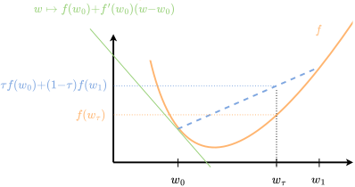
凸函数是指这样的函数:它在两个或更多点的平均值处的取值,小于这些点处函数值的平均值。图 15.3 对此作了图示,下面给出形式化表述。A convex function is a function such that its value on the average of two or more points is smaller than the average of the values of the functions at these points. This is illustrated in Figure 15.3 and formalized below.
定义 15.4.8(凸函数)。Definition 15.4.8 (Convex functions).
上述刻画可以很容易地推广到多个点。具体而言,对 与 ,若 (即 定义了 上的一个概率分布),则当 为凸函数时,有The above characterization can easily be generalized to multiple points. Namely, for and such that (that is, defines a probability distribution over , we have if is convex that
点 称为凸组合。这可以看作是把函数在平均点处的取值与这些点处函数值的平均值进行比较,并且可以进一步推广到任意随机变量。The point is called a convex combination. This can be seen as comparing the function at the average point to the average of the values at these points and can further be generalized to any random variable.
命题 15.4.9(Jensen 不等式)。Proposition 15.4.9 (Jensen’s inequality).
若所考虑的函数可微,则凸性还有一种刻画方式:考察该函数的线性近似如何从下方界定该函数。图 15.3 对此作了图示,下面给出形式化表述。If the function considered is differentiable, an alternative characterization of convexity is to observe how linear approximations of the function lower bound the function. This is illustrated in Figure 15.3 and formalized below.
定义 15.4.10(凸的可微函数)。Definition 15.4.10 (Convex differentiable functions).
上述刻画点明了凸函数在优化中的重要性:如果我们能找到一个梯度为零的点 ,那么我们就知道已经找到了最小值,因为此时有The above characterization pinpoints the relevance of convex functions in optimization: if we can find a point with null gradient, then we know that we have found the minimum as we have
这意味着,只要能够获得函数的梯度或梯度的近似,我们就有了一个充分判据,用以判断是否找到了全局最小值。在对光滑函数进行梯度下降的情形下,凸性保证以次线性速率收敛到最小值,具体如下所述。This means that by having access to the gradient of the function or an approximation thereof, we have access to a sufficient criterion to know whether we found a global minimum. In the case of a gradient descent on a smooth function, convexity ensures convergence to a minimum at a sublinear rate as detailed below.
最后,若函数二次可微,则函数的凸性可以用该函数的 Hessian 矩阵来刻画。Finally, if the function is twice differentiable, convexity of a function can be characterized in terms of the Hessian of the function.
命题 15.4.11(凸的二次可微函数)。Proposition 15.4.11 (Convex twice differentiable functions).
15.4.4 强凸函数Strongly-convex functions
凸性也可以通过考虑 -强凸函数来加强。Convexity can also be strengthened by considering -strongly convex functions.
定义 15.4.12(强凸函数)。Definition 15.4.12 (Strongly-convex functions).
关于可微函数的强凸性刻画指出, 被一个二次函数从下方界定。这使得我们能够设计具有线性收敛性的算法,后文将对此加以说明。我们自然地有如下蕴含关系The characterization of strong convexity for differentiable functions states that is lower-bounded by a quadratic. This enables the design of linearly convergent algorithms as explained later. We naturally have the implications
关于任意范数With respect to arbitrary norms
一个函数可以关于任意范数强凸,只需将定义 15.4.12 中的 -范数换成该范数即可。对于可微的强凸函数,我们还有如下另一种刻画,它将定义 15.4.12 推广到了任意范数。A function can be strongly convex w.r.t. an arbitrary norm, simply by replacing the -norm in Definition 15.4.12 with that norm. For differentiable strongly convex functions, we have the following alternative characterization, generalizing Definition 15.4.12 to arbitrary norms.
命题 15.4.13(可微的强凸函数)。Proposition 15.4.13 (Differentiable strongly-convex functions).
显而易见,若函数 是 -强凸的,则 是 -强凸的。由于所有范数彼此等价,一个函数若关于某一范数强凸,则它关于另一范数也必然强凸。不过,明确指出强凸性所依据的范数,往往能给出更好的常数 (就例如梯度下降的收敛速率而言,该常数越大越好)。我们还要强调,指明强凸性在哪个集合上成立同样十分重要。下面给出几个例子。Obviously, if a function is -strongly convex, then, is -strongly convex. Because all norms are equivalent, if a function is strongly convex w.r.t. a norm, it is also strongly-convex w.r.t. another norm. However, stating the norm w.r.t. which strong convexity holds can lead to better constant (the higher, the better in terms of convergence rates of, e.g., a gradient descent). We also emphasize that it is important to mention over which set strong convexity holds. We give examples below.
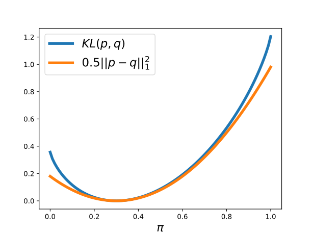
例 15.4.14(强凸函数)。Example 15.4.14 (Strongly convex functions).
15.4.5 非凸函数Nonconvex functions
一般而言,函数的最小值点必然具有零梯度,即In general, the minimum of a function necessarily has a null gradient, that is,
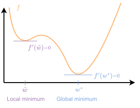
为看清这一点,考虑函数 。若 ,则 。因此存在一个很小的 ,使得 ,也就是 并非最小值点。然而,若函数不是凸的,其逆命题先验地并不成立:找到一个梯度为零的点,并不足以保证我们已经找到了全局最小值,如图 15.3 所示。To see this, consider the function . If , then . Therefore, there exists a small such that , i.e., is not the minimum. However, if the function is not convex, the converse is a priori not true: finding a point that has a null gradient does not ensure that we have found a global minimum as illustrated in Figure 15.3.
对于非凸函数,梯度为零的点称为驻点。驻点可能对应局部极大值,也可能对应局部极小值。形式上, 是局部极小值点,当For non-convex functions, a point with null gradient is called a stationary point. A stationary point may define a local maximum or a local minimum. Formally, is a local minimum if
局部极大值的定义与此类似,只是要求 的某个邻域内 。因此,对于非凸函数,收敛速率通常以梯度范数 趋于 的收敛性来表示。这类理论结果并不能保证收敛到全局最小值,而只能保证收敛到这样一点:仅凭梯度信息,先验地可能无法再取得任何进展。A local maximum is defined similarly, except that in a neighborhood of . For non-convex functions, convergence rates are therefore generally expressed in terms of convergence of the norm of the gradient towards . Such theoretical results do not ensure convergence to the global minimum but rather convergence to a point where no further progress may a priori be possible with just gradient information.
15.5 性能保证15.5 Performance guarantees
对于给定的函数类,我们可以把算法的性能定义为:该算法找到一个如式 15.1 所示的 -精确解所需的迭代次数。这称为算法的计算复杂度,记为For a given class of functions, we can define the performance of an algorithm as the number of iterations the algorithm would need to find an -accurate solution as in Eq. 15.1. This is called the computational complexity of the algorithm, denoted
或者,算法的性能也可以用收敛速率来表述,即在 次迭代后算法所达到的精度,Alternatively, the performance of an algorithm can be stated in terms of convergence rate, i.e., the accuracy that the algorithm reaches after iterations,
其中 是一个随 趋于零的递减正函数。通常, 会包含被极小化的函数的性质(例如其光滑性常数 ),以及关于初始点的信息(例如其函数值)。相应地,计算复杂度 则定义为满足 所需的最小迭代次数 ,where is a decreasing positive function vanishing as . Usually, incorporates properties of the function minimized, such as its smoothness constant and information on the initial point, such as its function value. The corresponding computational complexity is then given as the minimum number of iterations such that ,
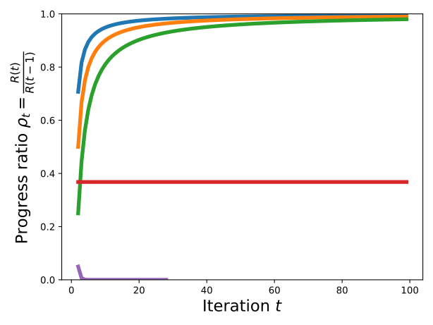
收敛速率一般可以通过考察第 次迭代的进展比来分类,该比值定义为Convergence rates can generally be classified by considering the progress ratio on iteration , defined by
渐近收敛速率则定义为The asymptotic convergence rate is then defined by
我们可以按如下方式对速率进行分类。We can classify the rates as follows.
- 1.
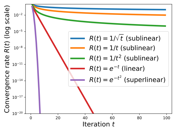
次线性收敛速率,:算法运行得越久,进展越慢。也就是说,随着 ,相对进展最终趋于停滞。属于这一类的 的例子包括 ,或者更一般地,对某个 有 。这等价于 。Sublinear convergence rates, : the longer the algorithm runs, the slower it makes progress. That is, the relative progress eventually tends to stall as . Examples of in this category include or more generally for some . This is equivalent to .
- 2.
线性收敛速率,:算法最终会在每次迭代时达到恒定的相对进展状态,从而给出 的总体速率 ,具体取决于目标函数的性质。这对应 。Linear convergence rates, : the algorithm eventually reaches a state of constant relative progress at each iteration, leading to an overall rate for depending on the properties of the objective. This corresponds to .
- 3.
超线性收敛速率,:每次新的迭代中相对进展都更好。例如, 时便可能发生这种情况,从而导致 ;或者 ,这专门称为二次速率,会导致 。Superlinear convergence rates, : the relative progress is better at each new iteration. This can happen for, e.g., , leading to , or , which is specifically called a quadratic rate, leading to .
这一点如图 15.4 所示。This is illustrated in Fig. 15.4.
注意,“线性”一词可能引起误解,因为这些速率实际上按指数方式变化。它们之所以被称为“线性”,是因为其在对数尺度下的表现。Note that the term “linear” may be misleading as the rates are in fact exponential. They are called “linear” because of their behavior in log scale.
上界与下界Upper and lower bounds
一类算法在给定 oracle(例如一阶 oracle)下所能达到的最佳性能,可以由上界或下界来刻画。由此可以证明:一个只能访问某一类 oracle 的算法,在理论上不可能优于某个数值。例如,对于限制在 上的 -光滑函数,使用一阶 oracle 进行极小化的计算复杂度下界为 [143, 1.1.7]。例如,取 和 时,这给出 次迭代。注意,这些结果在构造上就是悲观的。对于该函数类的某个具体实例,算法的实际性能可能远好于这种最坏情形——诸如拟牛顿法之类的常用算法便是如此。通过进一步把函数类限制为凸函数,可以获得更好的计算复杂度;凸函数在优化以及许多其他领域中扮演着核心角色。The best performance of a class of algorithms equipped with a given oracle (e.g. first-order oracle) can be upper-bounded or lower-bounded. This allows to show that an algorithm with access limited to a certain type of oracle cannot theoretically do better than a certain number. For example, the computational complexity to minimize -smooth functions restricted on with first-order oracles is lower bounded by [143, 1.1.7]. For example, with and , this gives iterations. Note that these results are pessimistic by construction. The actual performance of an algorithm on a specific instance of this function class may be much better than this worst-case scenario, as it is the case with popular algorithms such as quasi-Newton methods. Better computational complexities can be achieved by further restricting the class of functions to the set of convex functions, which play a central role in optimization and many other fields.
零阶与一阶Zero-order vs. first-order
对于光滑强凸函数类,最佳一阶算法的计算复杂度(在常数因子和对数因子意义下)比最佳零阶算法好 倍 [146, 147]。这一理论比较表明:虽然对于低维问题 ,零阶优化算法的表现可能与一阶优化算法相当,但对于高维问题,即 ,它们可能慢得多。For the class of smooth strongly convex functions, the computational complexity of the best first-order algorithm is (up to constant and logarithmic factors) times better than that of the best zero-order algorithm [146, 147]. This theoretical comparison shows that, while zero-order optimization algorithms may perform on par with first-order optimization algorithms for problems with a low dimension , they can be much slower for high dimensional problems, i.e., .
在不同的设定下,例如使用随机 oracle [58] 或针对不同的函数类,可能会得到略有不同的比较结果,例如以 因子代替 。然而,在当前所考虑的框架中,同样的结论依然成立:一阶优化算法能够给出与维数无关的快速速率,而零阶优化算法的速率通常依赖于问题的维数,因此不适合高维问题。In different settings, for example with stochastic oracles [58] or for different classes of functions, slightly different comparisons may be achieved, such as a factor instead of . However, the same conclusion holds in the current frameworks considered: first-order optimization algorithms can provide fast rates that are dimension independent while the rates of zero-order optimization algorithms generally depend on the dimension of the problem, making them unfit for high-dimensional problems.
这解释了一阶算法在训练神经网络方面取得的巨大成功。幸运的是,借助第 8 章所研究的反向模式自动微分,可以证明计算梯度的复杂度与计算函数本身的复杂度大致相同(见 8.3.3 节)。This explains the immense success of first-order algorithms for training neural networks. Fortunately, using reverse-mode autodiff, as studied in Chapter 8, it can be shown that computing a gradient has roughly the same complexity as evaluating the function itself Section 8.3.3.
15.6 小结15.6 Summary
- •
我们所能获得的关于某个函数的信息,可以用 oracle 这一概念来形式化。零阶 oracle 只能对函数求值;一阶 oracle 还能计算梯度;二阶 oracle 还能计算Hessian 矩阵或Hessian 矩阵—向量乘积(HVP)。The information available to us on a function can be formalized by the notion of oracle. Zero-order oracles can only evaluate the function; first-order oracles can also compute the gradient; second-order oracles can also compute the Hessian or the Hessian-vector product (HVP).
- •
本书回顾的大多数优化算法都可以从变分视角来看待:在这一视角下,下一次迭代是通过在函数近似与邻近项之间进行权衡优化而产生的。不同的近似方式与不同的邻近项会导出不同的算法。Most optimization algorithms reviewed in this book can be viewed from a variational perspective, in which the next iteration is produced by optimizing a trade-off between an approximation of the function and a proximity term. Different approximations and different proximity terms lead to different algorithms.
- •
我们还回顾了不同的函数类以及性能保证。We also reviewed different classes of functions, and performance guarantees.