第 18 章对偶性

18.1 对偶范数18.1 Dual norms

本节引入对偶范数，因为它们在本书中很有用。We introduce in this section dual norms, since they are useful in this book.

定义 18.1.1（对偶范数）。Definition 18.1.1 (Dual norms).

给定范数

\|{\bm{u}}\|

，其对偶范数为Given a norm

\|{\bm{u}}\|

, its dual is

\|{\bm{v}}\|_{*}\coloneqq\max_{\|{\bm{u}}\|\leq 1}\langle{\bm{u}},{\bm{v}}\rangle.

B_{\|\cdot\|}\coloneqq\{{\bm{u}}\in\mathbb{R}^{D}\colon\|{\bm{u}}\|\leq 1\}.

下面给出若干对偶范数对的例子。We give examples of pairs of dual norms below.

例 18.1.2（ $p$ -范数的对偶范数）。Example 18.1.2 (Dual norm of $p$ -norms).

p

-范数定义为The

p

-norm is defined by

\|{\bm{u}}\|_{p}\coloneqq\left(\sum_{j=1}^{D}|u_{j}|^{p}\right)^{1/p}.

其对偶为

\|{\bm{v}}\|_{q}

，其中

q

满足

\frac{1}{p}+\frac{1}{q}=1

。例如，

2

-范数的对偶范数就是它本身，因为

\frac{1}{2}+\frac{1}{2}=1

。

1

-范数与

\infty

-范数互为对偶，因为

\frac{1}{1}+\frac{1}{\infty}=1

。Its dual is

\|{\bm{v}}\|_{q}

where

q

is such that

\frac{1}{p}+\frac{1}{q}=1

. For instance, the dual norm of the

2

-norm is itself, since

\frac{1}{2}+\frac{1}{2}=1

. The

1

-norm and the

\infty

-norm are duals of each other, since

\frac{1}{1}+\frac{1}{\infty}=1

.

对偶范数的定义蕴含了柯西—施瓦茨不等式的一种推广：对于所有 ${\bm{u}},{\bm{v}}\in\mathbb{R}^{D}$ The definition of dual norm implies a generalization of the Cauchy–Schwarz inequality: for all ${\bm{u}},{\bm{v}}\in\mathbb{R}^{D}$

|\langle{\bm{u}},{\bm{v}}\rangle|\leq\|{\bm{u}}\|_{*}\|{\bm{v}}\|.

参见，例如，[18, 引理 1.4]。See, e.g., [18, Lemma 1.4].

命题 18.1.3（范数与平方范数的共轭）。Proposition 18.1.3 (Conjugate of norms and squared norms).

我们知道，支撑函数的共轭即指示函数。因此，若

f({\bm{u}})=\|{\bm{u}}\|

，则We know that the conjugate of the support function is the indicator function. Therefore, if

f({\bm{u}})=\|{\bm{u}}\|

, then

f^{*}({\bm{v}})=\iota_{B_{\|\cdot\|}}({\bm{v}})=\begin{cases}0&\text{ if }\|{\bm{v}}\|_{*}\leq 1\\ \infty&\text{ otherwise }\end{cases}.

另一方面，若

f({\bm{u}})=\frac{1}{2}\|{\bm{u}}\|^{2}

，则On the other hand, if

f({\bm{u}})=\frac{1}{2}\|{\bm{u}}\|^{2}

, then

f^{*}({\bm{v}})=\frac{1}{2}\|{\bm{v}}\|^{2}_{*}.

18.2 Fenchel 对偶18.2 Fenchel duality

本节考虑如下形式的标准目标函数We consider in this section standard objectives of the form

\min_{{\bm{w}}\in\mathcal{W}}L({\bm{w}})\coloneqq\min_{{\bm{w}}\in\mathcal{W}}\ell(f({\bm{w}}))+R({\bm{w}}),

其中 $f\colon\mathcal{W}\to\mathcal{M}$ 、 $\ell\colon\mathcal{M}\to\mathbb{R}$ 与 $R\colon\mathcal{W}\to\mathbb{R}$ 。我们首先说明：即使原始问题是非凸的，该目标函数的极小化（称为原始问题）仍可被一个称为对偶的凹极大化目标函数从下方界定。where $f\colon\mathcal{W}\to\mathcal{M}$ , $\ell\colon\mathcal{M}\to\mathbb{R}$ and $R\colon\mathcal{W}\to\mathbb{R}$ . We first show that the minimization of this objective, called the primal, can be lower bounded by a concave maximization objective, called the dual, even if the primal is nonconvex.

命题 18.2.1（弱对偶性）。Proposition 18.2.1 (Weak duality).

设

f\colon\mathcal{W}\to\mathcal{M}

（可能非线性）、

\ell\colon\mathcal{M}\to\mathbb{R}

（可能非凸）以及

R\colon\mathcal{W}\to\mathbb{R}

（可能非凸）。则Let

f\colon\mathcal{W}\to\mathcal{M}

(potentially nonlinear),

\ell\colon\mathcal{M}\to\mathbb{R}

(potentially nonconvex) and

R\colon\mathcal{W}\to\mathbb{R}

(potentially nonconvex). Then

\min_{{\bm{w}}\in\mathcal{W}}\ell(f({\bm{w}}))+R({\bm{w}})\geq\max_{{\bm{\alpha}}\in\mathcal{M}}-R^{f}({\bm{\alpha}})-\ell^{*}(-{\bm{\alpha}}),

其中我们使用了共轭where we used the conjugate

\ell^{*}(-{\bm{\alpha}})\coloneqq\max_{{\bm{\theta}}\in\mathcal{M}}\langle-{\bm{\alpha}},{\bm{\theta}}\rangle-\ell({\bm{\theta}})

以及“广义共轭”and the “generalized conjugate”

R^{f}({\bm{\alpha}})\coloneqq\max_{{\bm{w}}\in\mathcal{W}}\langle{\bm{\alpha}},f({\bm{w}})\rangle-R({\bm{w}}).

此外，

\ell^{*}

与

R^{f}

均为凸函数。Moreover,

\ell^{*}

and

R^{f}

are both convex functions.

我们强调，命题 18.2.1 中的结果具有完全的一般性，即它并不假设 $f$ 的线性性，也不假设 $\ell$ 与 $R$ 的凸性。当然需要注意的是，若 $f$ 是非线性的，且 $\ell$ 与 $R$ 是非凸的，则 $R^{f}$ 与 $\ell^{*}$ 一般难以计算。We emphasize that the result in Proposition 18.2.1 is fully general, in the sense that it does not assume the linearity of $f$ or the convexity of $\ell$ and $R$ . The caveat, of course, is that $R^{f}$ and $\ell^{*}$ are difficult to compute in general, if $f$ is nonlinear, and if $\ell$ and $R$ are nonconvex.

证明 18.2.2。Proof 18.2.2.

	$\displaystyle\min_{{\bm{w}}\in\mathcal{W}}\ell(f({\bm{w}}))+R({\bm{w}})$
$\displaystyle=$	$\displaystyle\min_{\begin{subarray}{c}{\bm{w}}\in\mathcal{W}\\ {\bm{\theta}}\in\mathcal{M}\end{subarray}}\ell({\bm{\theta}})+R({\bm{w}})\quad\text{s.t.}\quad{\bm{\theta}}=f({\bm{w}})$
$\displaystyle=$	$\displaystyle\min_{\begin{subarray}{c}{\bm{w}}\in\mathcal{W}\\ {\bm{\theta}}\in\mathcal{M}\end{subarray}}\max_{{\bm{\alpha}}\in\mathcal{M}}\ell({\bm{\theta}})+R({\bm{w}})+\langle{\bm{\alpha}},{\bm{\theta}}-f({\bm{w}})\rangle$
$\displaystyle\geq$	$\displaystyle\max_{{\bm{\alpha}}\in\mathcal{M}}\min_{\begin{subarray}{c}{\bm{w}}\in\mathcal{W}\\ {\bm{\theta}}\in\mathcal{M}\end{subarray}}\ell({\bm{\theta}})+R({\bm{w}})+\langle{\bm{\alpha}},{\bm{\theta}}-f({\bm{w}})\rangle$
$\displaystyle=$	$\displaystyle\max_{{\bm{\alpha}}\in\mathcal{M}}\min_{{\bm{w}}\in\mathcal{W}}\langle{\bm{\alpha}},-f({\bm{w}})\rangle+R({\bm{w}})+\min_{{\bm{\theta}}\in\mathcal{M}}\ell({\bm{\theta}})+\langle{\bm{\alpha}},{\bm{\theta}}\rangle$
$\displaystyle=$	$\displaystyle\max_{{\bm{\alpha}}\in\mathcal{M}}-\max_{{\bm{w}}\in\mathcal{W}}\langle{\bm{\alpha}},f({\bm{w}})\rangle-R({\bm{w}})-\max_{{\bm{\theta}}\in\mathcal{M}}\langle-{\bm{\alpha}},{\bm{\theta}}\rangle-\ell({\bm{\theta}})$
$\displaystyle=$	$\displaystyle\max_{{\bm{\alpha}}\in\mathcal{M}}-R^{f}({\bm{\alpha}})-\ell^{*}(-{\bm{\alpha}}).$

当 $f({\bm{w}})=A{\bm{w}}$ （其中 $A$ 是线性映射），且 $\ell$ 与 $R$ 均为凸时，我们可以得到一个强得多的结果。In the case when $f({\bm{w}})=A{\bm{w}}$ , where $A$ is a linear map, and when both $\ell$ and $R$ are convex, we can state a much stronger result.

命题 18.2.3（强对偶性）。Proposition 18.2.3 (Strong duality).

设

A

为从

\mathcal{W}

到

\mathcal{M}

的线性映射，

\ell\colon\mathcal{M}\to\mathbb{R}

与

R\colon\mathcal{W}\to\mathbb{R}

为凸函数，

A^{*}

表示

A

的伴随（见第 2.3 节）。则Let

A

be a linear map from

\mathcal{W}

to

\mathcal{M}

. Let

\ell\colon\mathcal{M}\to\mathbb{R}

and

R\colon\mathcal{W}\to\mathbb{R}

be convex functions. Let

A^{*}

denote the adjoint of

A

(Section 2.3). Then,

\min_{{\bm{w}}\in\mathcal{W}}\ell(A{\bm{w}})+R({\bm{w}})=\max_{{\bm{\alpha}}\in\mathcal{M}}-R^{*}(A^{*}{\bm{\alpha}})-\ell^{*}(-{\bm{\alpha}}).

此外，原问题的解满足Furthermore, the primal solution satisfies

{\bm{w}}^{\star}\in\argmax_{{\bm{w}}\in\mathcal{W}}\langle A{\bm{\alpha}}^{\star},{\bm{w}}\rangle-R({\bm{w}}).

当

R

为严格凸时，原问题的解由下式唯一确定：When

R

is strictly convex, the primal solution is uniquely determined by

{\bm{w}}^{\star}=\nabla R^{*}(A^{*}{\bm{\alpha}}^{\star}).

证明 18.2.4。Proof 18.2.4.

由 $f({\bm{w}})=A{\bm{w}}$ ，可得Since $f({\bm{w}})=A{\bm{w}}$ , we have

$\displaystyle R^{f}({\bm{\alpha}})$	$\displaystyle\coloneqq\max_{{\bm{w}}\in\mathcal{W}}\langle{\bm{\alpha}},f({\bm{w}})\rangle-R({\bm{w}})$
	$\displaystyle=\max_{{\bm{w}}\in\mathcal{W}}\langle{\bm{\alpha}},A{\bm{w}}\rangle-R({\bm{w}})$
	$\displaystyle=\max_{{\bm{w}}\in\mathcal{W}}\langle A^{*}{\bm{\alpha}},{\bm{w}}\rangle-R({\bm{w}})$
	$\displaystyle=R^{}(A^{}{\bm{\alpha}}).$

此外，命题18.2.1的证明中的不等式取等号，因为 $\min\max$ 是某个凸—凹函数的对应量。Furthermore, the inequality in the proof of Proposition 18.2.1 is an equality, since the $\min\max$ is that of a convex-concave function.

命题 18.2.3 中的极大化问题称为 Fenchel 对偶。由强对偶性可知，最大值与最小值相等。因此，我们可以等价地选择求解对偶问题，而非原始问题。当空间 $\mathcal{M}$ 小于 $\mathcal{W}$ 时，这样做尤为有利。The maximization problem in Proposition 18.2.3 is called the Fenchel dual. By strong duality, the value of the maximum and the value of the minimum are equal. We can therefore choose to equivalently solve the dual instead of the primal. This can be advantageous when the space $\mathcal{M}$ is smaller than $\mathcal{W}$ .

下面我们应用 Fenchel 对偶，得到正则化多分类线性分类问题的对偶。We now apply the Fenchel dual to obtain the dual of regularized multiclass linear classification.

例 18.2.5（可分离损失函数之和）。Example 18.2.5 (Sum of separable loss functions).

当损失为

\ell({\bm{\theta}})\coloneqq\sum_{i=1}^{N}\ell_{i}({\bm{\theta}}_{i})

时，其中

{\bm{\theta}}=A{\bm{w}}=(A_{1}{\bm{w}},\dots,A_{N}{\bm{w}})\in\mathcal{M}^{N}

，而

A_{i}

为从

\mathcal{W}

到

\mathcal{M}

的线性映射，可得When the loss is

\ell({\bm{\theta}})\coloneqq\sum_{i=1}^{N}\ell_{i}({\bm{\theta}}_{i})

, where

{\bm{\theta}}=A{\bm{w}}=(A_{1}{\bm{w}},\dots,A_{N}{\bm{w}})\in\mathcal{M}^{N}

and

A_{i}

is a linear map from

\mathcal{W}

to

\mathcal{M}

, we obtain

\min_{{\bm{w}}\in\mathcal{W}}\sum_{i=1}^{N}\ell_{i}(A_{i}{\bm{w}})+R({\bm{w}})=\max_{{\bm{\alpha}}\in\mathcal{M}^{N}}-R^{*}(A^{*}{\bm{\alpha}})-\sum_{i=1}^{N}\ell_{i}^{*}(-{\bm{\alpha}}_{i}),

其中

A^{*}{\bm{\alpha}}=(A_{1}^{*}{\bm{\alpha}}_{1},\dots,A_{N}^{*}{\bm{\alpha}}_{N})

。通常，我们定义where

A^{*}{\bm{\alpha}}=(A_{1}^{*}{\bm{\alpha}}_{1},\dots,A_{N}^{*}{\bm{\alpha}}_{N})

. Typically, we define

A_{i}{\bm{w}}\coloneqq{\bm{W}}{\bm{x}}_{i},

其中

{\bm{W}}\in\mathbb{R}^{M\times D}

是

{\bm{w}}\in\mathcal{W}

经重塑后的版本，

{\bm{x}}_{i}\in\mathbb{R}^{D}

为一个训练样本，

M

为类别数。此时可得where

{\bm{W}}\in\mathbb{R}^{M\times D}

is a reshaped version of

{\bm{w}}\in\mathcal{W}

,

{\bm{x}}_{i}\in\mathbb{R}^{D}

is a training sample, and

M

is the number of classes. In this case, we then have

A_{i}^{*}{\bm{\alpha}}_{i}={\bm{\alpha}}_{i}{\bm{x}}_{i}^{\top}.

损失函数的共轭示例见表 18.1。Examples of loss function conjugates are given in Table 18.1.

表 18.1：损失共轭的示例。对于回归损失（平方损失、绝对损失），其中

{\bm{y}}_{i}\in\mathbb{R}^{M}

，我们定义

{\bm{t}}_{i}=\phi({\bm{y}}_{i})={\bm{y}}_{i}

。对于分类损失（logistic 损失、感知机损失、合页损失），其中

y_{i}\in[M]

，我们定义

{\bm{t}}_{i}=\phi(y_{i})={\bm{e}}_{y_{i}}

。为简化部分表达式，我们作了变量替换

{\bm{\mu}}_{i}\coloneqq{\bm{y}}_{i}-{\bm{\alpha}}_{i}

。Table 18.1: Examples of loss conjugates. For regression losses (squared, absolute), where

{\bm{y}}_{i}\in\mathbb{R}^{M}

, we define

{\bm{t}}_{i}=\phi({\bm{y}}_{i})={\bm{y}}_{i}

. For classification losses (logistic, perceptron, hinge), where

y_{i}\in[M]

, we define

{\bm{t}}_{i}=\phi(y_{i})={\bm{e}}_{y_{i}}

. To simplify some expressions, we defined the change of variable

{\bm{\mu}}_{i}\coloneqq{\bm{y}}_{i}-{\bm{\alpha}}_{i}

.

	$\ell_{i}({\bm{\theta}}_{i})$	$\ell_{i}^{*}(-{\bm{\alpha}}_{i})$
平方Squared	$\frac{1}{2}\\|{\bm{\theta}}_{i}-{\bm{t}}_{i}\\|^{2}_{2}$	$\frac{1}{2}\\|{\bm{\alpha}}_{i}\\|^{2}_{2}-\langle{\bm{t}}_{i},{\bm{\alpha}}_{i}\rangle$
绝对Absolute	$\\|{\bm{\theta}}_{i}-{\bm{t}}_{i}\\|_{1}$	$\iota_{[-1,1]^{M}}({\bm{\alpha}}_{i})-\langle{\bm{t}}_{i},{\bm{\alpha}}_{i}\rangle$
logisticLogistic	$\mathrm{LSE}({\bm{\theta}}_{i})-\langle{\bm{\theta}}_{i},{\bm{t}}_{i}\rangle$	$\langle{\bm{\mu}}_{i},\log{\bm{\mu}}_{i}\rangle+\iota_{\triangle^{M}}({\bm{\mu}}_{i})$
感知机Perceptron	$\max_{j\in[M]}\theta_{i,j}-\theta_{i,y_{i}}$	$\iota_{\triangle^{M}}({\bm{\mu}}_{i})$
合页Hinge	$\max_{j\in[M]}[j\neq y_{i}]+\theta_{i,j}-\theta_{i,y_{i}}$	$\iota_{\triangle^{M}}({\bm{\mu}}_{i})-\langle\operatorname{\mathbf{1}}-{\bm{t}}_{i},{\bm{\mu}}_{i}\rangle$

18.3 Bregman 散度18.3 Bregman divergences

Bregman 散度用于度量两点之间的差异。Bregman divergences are a measure of difference between two points.

定义 18.3.1（Bregman 散度）。Definition 18.3.1 (Bregman divergence).

由可微凸函数

f\colon\mathbb{R}^{D}\to\mathbb{R}

生成的 Bregman 散度为The Bregman divergence generated by a differentiable convex function

f\colon\mathbb{R}^{D}\to\mathbb{R}

is

\displaystyle B_{f}({\bm{u}},{\bm{v}})

\displaystyle\coloneqq f({\bm{u}})-f({\bm{v}})-\langle\nabla f({\bm{v}}),{\bm{u}}-{\bm{v}}\rangle

\displaystyle=\langle\nabla f({\bm{v}}),{\bm{v}}\rangle-f({\bm{v}})-\left[\langle\nabla f({\bm{v}}),{\bm{u}}\rangle-f({\bm{u}})\right],

其中

{\bm{u}},{\bm{v}}\in\dom(f)

。where

{\bm{u}},{\bm{v}}\in\dom(f)

.

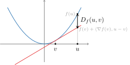
直观地说，Bregman 散度是 $f({\bm{u}})$ 与其在 ${\bm{v}}$ 附近的线性化 ${\bm{u}}\mapsto f({\bm{v}})+\langle\nabla f({\bm{v}}),{\bm{u}}-{\bm{v}}\rangle$ 之差。这一点如图 18.1 所示。Intuitively, the Bregman divergence is the difference between $f({\bm{u}})$ and its linearization ${\bm{u}}\mapsto f({\bm{v}})+\langle\nabla f({\bm{v}}),{\bm{u}}-{\bm{v}}\rangle$ around ${\bm{v}}$ . This is illustrated in Fig. 18.1.

例 18.3.2（Bregman 散度的示例）。Example 18.3.2 (Examples of Bregman divergences).

若

f({\bm{u}})=\frac{1}{2}\|{\bm{u}}\|^{2}_{2}

，其中

\dom(f)=\mathbb{R}^{D}

，则得到If

f({\bm{u}})=\frac{1}{2}\|{\bm{u}}\|^{2}_{2}

, where

\dom(f)=\mathbb{R}^{D}

, then

B_{f}({\bm{u}},{\bm{v}})=\frac{1}{2}\|{\bm{u}}-{\bm{v}}\|^{2}_{2},

平方欧几里得距离。若

f({\bm{u}})=\langle{\bm{u}},\log{\bm{u}}\rangle

，其中

\dom(f)=\mathbb{R}_{+}^{D}

，则得到the squared Euclidean distance. If

f({\bm{u}})=\langle{\bm{u}},\log{\bm{u}}\rangle

, where

\dom(f)=\mathbb{R}_{+}^{D}

, then

B_{f}({\bm{u}},{\bm{v}})=\sum_{j=1}^{D}u_{j}\log\frac{u_{j}}{v_{j}}-\sum_{j=1}^{D}u_{j}+\sum_{j=1}^{D}v_{j},

（广义）Kullback-Leibler 散度。the (generalized) Kullback-Leibler divergence.

性质Properties

Bregman 散度具有若干有用的性质。Bregman divergences enjoy several useful properties.

命题 18.3.3（Bregman 散度的性质）。Proposition 18.3.3 (Properties of Bregman divergences).

设

f\colon\mathbb{R}^{D}\to\mathbb{R}

为可微凸函数。Let

f\colon\mathbb{R}^{D}\to\mathbb{R}

be a differentiable convex function. 1. 非负性：对任意

{\bm{u}},{\bm{v}}\in\dom(f)

，均有

B_{f}({\bm{u}},{\bm{v}})\geq 0

。Non-negativity:

B_{f}({\bm{u}},{\bm{v}})\geq 0

for all

{\bm{u}},{\bm{v}}\in\dom(f)

. 2. 正性：

B_{f}({\bm{u}},{\bm{v}})=0

当且仅当

{\bm{u}}={\bm{v}}

（此时

f

为严格凸）。Positivity:

B_{f}({\bm{u}},{\bm{v}})=0

if and only if

{\bm{u}}={\bm{v}}

(when

f

is strictly convex). 3. 凸性：

B_{f}({\bm{u}},{\bm{v}})

关于

{\bm{u}}

是凸的。Convexity:

B_{f}({\bm{u}},{\bm{v}})

is convex in

{\bm{u}}

. 4. 对偶空间形式：

B_{f}({\bm{u}},{\bm{v}})=B_{f^{*}}({\bm{b}},{\bm{a}})

，其中

{\bm{b}}=\nabla f({\bm{v}})\in\dom(f^{*})

，

{\bm{a}}=\nabla f({\bm{u}})\in\dom(f^{*})

。Dual-space form:

B_{f}({\bm{u}},{\bm{v}})=B_{f^{*}}({\bm{b}},{\bm{a}})

, where

{\bm{b}}=\nabla f({\bm{v}})\in\dom(f^{*})

and

{\bm{a}}=\nabla f({\bm{u}})\in\dom(f^{*})

.

证明 18.3.4。Proof 18.3.4.

这些性质均可由 $f({\bm{u}})$ 的凸性直接得到。The properties follow immediately from the convexity of $f({\bm{u}})$ .

1.

由定义 15.4.10 即得。From Definition 15.4.10.
2.

由极小值点的唯一性即得。From the uniqueness of minimizers.
3.

这源于如下事实： ${\bm{u}}\mapsto B_{f}({\bm{u}},{\bm{v}})$ 是 $f({\bm{u}})$ 与 ${\bm{u}}$ 的一个线性函数之和。From the fact that ${\bm{u}}\mapsto B_{f}({\bm{u}},{\bm{v}})$ is the sum of $f({\bm{u}})$ and a linear function of ${\bm{u}}$ .

图 18.1：由

f

生成的 Bregman 散度，即

f({\bm{u}})

与其在

{\bm{v}}

附近的线性化之差。Figure 18.1: The Bregman divergence generated by

f

is the difference between

f({\bm{u}})

and its linearization around

{\bm{v}}

.

Bregman 散度可用于定义欧几里得投影与邻近算子的自然推广；这些内容已在 16.3 节与 16.4 节中回顾。The Bregman divergence can be used to define natural generalizations of the Euclidean projection and proximal operators, reviewed in Section 16.3 and Section 16.4.

定义 18.3.5（Bregman 邻近算子与投影算子）。Definition 18.3.5 (Bregman proximal and projection operators).

设

{\bm{v}}\in\dom(f)

。Bregman 近端算子为Let

{\bm{v}}\in\dom(f)

. The Bregman proximal operator is

\mathrm{bprox}_{f,g}({\bm{v}})\coloneqq\argmin_{{\bm{u}}\in\dom(f)\cap\dom(g)}B_{f}({\bm{u}},{\bm{v}})+g({\bm{u}}).

特别地，到

\mathcal{C}\subseteq\dom(f)

上的 Bregman 投影为In particular, the Bregman projection onto

\mathcal{C}\subseteq\dom(f)

is

\mathrm{bproj}_{f,\mathcal{C}}({\bm{v}})\coloneqq\argmin_{{\bm{u}}\in\mathcal{C}}B_{f}({\bm{u}},{\bm{v}}).

事实证明，这些算子与凸共轭的梯度映射密切相关。It turns out that these operators are intimately connected to the gradient mapping of the convex conjugate.

命题 18.3.6（与共轭的梯度的联系）。Proposition 18.3.6 (Link with conjugate’s gradient).

若

\Omega=f+g

，则对任意

{\bm{\theta}}\in\dom(f^{*})

，If

\Omega=f+g

, then for all

{\bm{\theta}}\in\dom(f^{*})

\nabla\Omega^{*}({\bm{\theta}})=\mathrm{bprox}_{f,g}(\nabla f^{*}({\bm{\theta}})).

特别地，若

\Omega=f+\iota_{\mathcal{C}}

，则对任意

{\bm{\theta}}\in\dom(f^{*})

，In particular, if

\Omega=f+\iota_{\mathcal{C}}

, then for all

{\bm{\theta}}\in\dom(f^{*})

\nabla\Omega^{*}({\bm{\theta}})=\mathrm{bproj}_{f,\mathcal{C}}(\nabla f^{*}({\bm{\theta}})).

下面给出两个例子。We give two examples below.

例 18.3.7（单纯形上的 Bregman 投影）。Example 18.3.7 (Bregman projections on the simplex).

若

f({\bm{u}})=\frac{1}{2}\|{\bm{u}}\|^{2}_{2}

，则If

f({\bm{u}})=\frac{1}{2}\|{\bm{u}}\|^{2}_{2}

, then

\displaystyle\mathrm{bproj}_{f,\triangle^{D}}({\bm{v}})=\argmin_{{\bm{u}}\in\triangle^{D}}\frac{1}{2}\|{\bm{u}}-{\bm{v}}\|^{2}_{2}.

若

f({\bm{u}})=\langle{\bm{u}},\log{\bm{u}}-\operatorname{\mathbf{1}}\rangle

，则If

f({\bm{u}})=\langle{\bm{u}},\log{\bm{u}}-\operatorname{\mathbf{1}}\rangle

, then

\displaystyle\mathrm{bproj}_{f,\triangle^{D}}({\bm{v}})=\argmin_{{\bm{u}}\in\triangle^{D}}\mathrm{KL}({\bm{u}},{\bm{v}})=\mathrm{softargmax}({\bm{\theta}}),

其中

{\bm{v}}=\nabla f^{*}({\bm{\theta}})=\exp({\bm{\theta}})

。where

{\bm{v}}=\nabla f^{*}({\bm{\theta}})=\exp({\bm{\theta}})

.

因此，softmax 可以看作是在 Kullback-Leibler 散度意义下向概率单纯形上的投影！Therefore, the softmax can be seen as a projection onto the probability simplex in the Kullback-Leibler divergence sense!

18.4 Fenchel-Young 损失函数18.4 Fenchel-Young loss functions

我们以对 Fenchel-Young 损失函数族 [28] 的简要回顾来结束本章，该损失函数族包含表 18.1 中的所有损失函数。We end this chapter with a brief review of the Fenchel-Young family of loss functions [28], which includes all loss functions in Table 18.1.

定义 18.4.1（Fenchel-Young 损失）。Definition 18.4.1 (Fenchel-Young loss).

由

\Omega

生成的 Fenchel-Young 损失函数为The Fenchel-Young loss function generated by

\Omega

is

\ell_{\Omega}({\bm{\theta}},{\bm{t}})\coloneqq\Omega^{*}({\bm{\theta}})+\Omega({\bm{t}})-\langle{\bm{\theta}},{\bm{t}}\rangle

其中

{\bm{\theta}}\in\dom(\Omega^{*})

，

{\bm{t}}\in\dom(\Omega)

。where

{\bm{\theta}}\in\dom(\Omega^{*})

and

{\bm{t}}\in\dom(\Omega)

.

通常，我们令 ${\bm{\theta}}=f({\bm{x}},{\bm{w}})$ ，其中 $f$ 是带有参数 ${\bm{w}}$ 的模型预测函数，且 ${\bm{t}}=\phi({\bm{y}})$ ，其中 $\phi\colon\mathcal{Y}\to\dom(\Omega)$ 。例如，假设我们处理的是分类输出 $y\in[M]$ 。那么，我们可以令 $\phi(y)={\bm{e}}_{y}$ ，其中 ${\bm{e}}_{y}$ 是 $y$ 的 one-hot 编码。Typically, we set ${\bm{\theta}}=f({\bm{x}},{\bm{w}})$ , where $f$ is a model prediction function with parameters ${\bm{w}}$ and ${\bm{t}}=\phi({\bm{y}})$ , where $\phi\colon\mathcal{Y}\to\dom(\Omega)$ . For instance, suppose we work with categorical outputs $y\in[M]$ . Then, we can set $\phi(y)={\bm{e}}_{y}$ , where ${\bm{e}}_{y}$ is the one-hot encoding of $y$ .

需要注意的重要一点是，Fenchel-Young 损失定义在混合空间中的变量上： ${\bm{\theta}}$ 属于对偶空间，而 ${\bm{t}}$ 属于原始空间。事实上，Fenchel-Young 损失与 Bregman 散度密切相关：若令 ${\bm{\theta}}=\nabla\Omega({\bm{v}})$ ，则 $B_{\Omega}({\bm{t}},{\bm{v}})=\Omega^{*}({\bm{\theta}})+\Omega({\bm{t}})-\langle{\bm{\theta}},{\bm{t}}\rangle$ 。Fenchel-Young 损失函数的关键性质总结如下。The important point to notice is that the Fenchel-Young loss is defined over arguments in mixed spaces: ${\bm{\theta}}$ belongs to the dual space, while ${\bm{t}}$ belongs to the primal space. In fact, the Fenchel-Young loss is intimately connected to the Bregman divergence, since $B_{\Omega}({\bm{t}},{\bm{v}})=\Omega^{*}({\bm{\theta}})+\Omega({\bm{t}})-\langle{\bm{\theta}},{\bm{t}}\rangle$ , if we set ${\bm{\theta}}=\nabla\Omega({\bm{v}})$ . The key properties of Fenchel-Young loss functions are summarized below.

命题 18.4.2（Fenchel-Young 损失函数的性质）。Proposition 18.4.2 (Properties of Fenchel-Young loss functions).

1. 非负性：对任意

{\bm{\theta}}\in\dom(\Omega^{*})

与

{\bm{t}}\in\dom(\Omega)

，均有

\ell_{\Omega}({\bm{\theta}},{\bm{t}})\geq 0

。Non-negativity:

\ell_{\Omega}({\bm{\theta}},{\bm{t}})\geq 0

for all

{\bm{\theta}}\in\dom(\Omega^{*})

and

{\bm{t}}\in\dom(\Omega)

. 2. 正性：若

\Omega

为严格凸函数，则

\ell_{\Omega}({\bm{\theta}},{\bm{t}})=0

当且仅当

\nabla\Omega^{*}({\bm{\theta}})={\bm{t}}

。Positivity:

\ell_{\Omega}({\bm{\theta}},{\bm{t}})=0

if and only if

\nabla\Omega^{*}({\bm{\theta}})={\bm{t}}

, assuming

\Omega

is strictly convex. 3. 凸性：

\ell_{\Omega}({\bm{\theta}},{\bm{t}})

关于

{\bm{\theta}}

为凸（无论

\Omega

如何），且当

\Omega

为凸时，关于

{\bm{t}}

亦为凸。Convexity:

\ell_{\Omega}({\bm{\theta}},{\bm{t}})

is convex in

{\bm{\theta}}

(regardless of

\Omega

) and in

{\bm{t}}

(if

\Omega

is convex). 4. 与复合 Bregman 散度的关系：Relation with composite Bregman divergence:

0\leq\underbrace{B_{\Omega}({\bm{t}},\nabla\Omega^{*}({\bm{\theta}}))}_{\text{possibly nonconvex in }{\bm{\theta}}}\leq\underbrace{\ell_{\Omega}({\bm{\theta}},{\bm{t}})}_{\text{convex in }{\bm{\theta}}}.

关于更多性质的深入研究，参见 [28]。See [28] for an in-depth study of more properties.

18.5 小结18.5 Summary

•

凸共轭是 Fenchel 对偶中的一个强大抽象工具，它将对偶表达式与特定于函数的项解耦。The convex conjugate serves as a powerful abstraction in Fenchel duality, decoupling the dual expression and function-specific terms.
•

凸共轭也与 Bregman 散度紧密相连，并可用于导出 Fenchel-Young 损失函数族，后者可以看作原始—对偶的 Bregman 散度。The convex conjugate is also tightly connected to Bregman divergences and can be used to derive the family of Fenchel-Young loss functions, which can be seen as primal-dual Bregman divergences.

第 18 章 对偶性Chapter 18 Duality

18.1 对偶范数18.1 Dual norms

定义 18.1.1（对偶范数）。Definition 18.1.1 (Dual norms).

例 18.1.2（ppp-范数的对偶范数）。Example 18.1.2 (Dual norm of ppp-norms).

命题 18.1.3（范数与平方范数的共轭）。Proposition 18.1.3 (Conjugate of norms and squared norms).

18.2 Fenchel 对偶18.2 Fenchel duality

命题 18.2.1（弱对偶性）。Proposition 18.2.1 (Weak duality).

证明 18.2.2。Proof 18.2.2.

命题 18.2.3（强对偶性）。Proposition 18.2.3 (Strong duality).

证明 18.2.4。Proof 18.2.4.

例 18.2.5（可分离损失函数之和）。Example 18.2.5 (Sum of separable loss functions).

18.3 Bregman 散度18.3 Bregman divergences

定义 18.3.1（Bregman 散度）。Definition 18.3.1 (Bregman divergence).

例 18.3.2（Bregman 散度的示例）。Example 18.3.2 (Examples of Bregman divergences).

性质Properties

命题 18.3.3（Bregman 散度的性质）。Proposition 18.3.3 (Properties of Bregman divergences).

证明 18.3.4。Proof 18.3.4.

定义 18.3.5（Bregman 邻近算子与投影算子）。Definition 18.3.5 (Bregman proximal and projection operators).

命题 18.3.6（与共轭的梯度的联系）。Proposition 18.3.6 (Link with conjugate’s gradient).

例 18.3.7（单纯形上的 Bregman 投影）。Example 18.3.7 (Bregman projections on the simplex).

18.4 Fenchel-Young 损失函数18.4 Fenchel-Young loss functions

定义 18.4.1（Fenchel-Young 损失）。Definition 18.4.1 (Fenchel-Young loss).

命题 18.4.2（Fenchel-Young 损失函数的性质）。Proposition 18.4.2 (Properties of Fenchel-Young loss functions).

18.5 小结18.5 Summary

第 18 章对偶性Chapter 18 Duality

例 18.1.2（ $p$ -范数的对偶范数）。Example 18.1.2 (Dual norm of $p$ -norms).