第 11 章通过优化求导 · Differentiating through optimization

11.1 隐函数11.1 Implicit functions

隐函数无法显式分解为初等函数，因而第 8 章所讨论的自动微分不能直接施用于其上。本章介绍对这类函数求导的技术，以及如何将其纳入自动微分框架。Implicit functions are functions that do not enjoy an explicit decomposition into elementary functions, for which automatic differentiation, as studied in Chapter 8, can therefore not be directly applied. We describe in this chapter techniques to differentiate through such functions and how to integrate them into an autodiff framework.

形式上，我们将隐函数记为 ${\bm{w}}^{\star}({\bm{\lambda}})$ ，其中 ${\bm{w}}^{\star}\colon\Lambda\to\mathcal{W}$ 。由此产生的一个问题是：如何计算雅可比矩阵 $\partial{\bm{w}}^{\star}({\bm{\lambda}})$ ？作为初步应用，可以考虑系统的灵敏度分析。例如， ${\bm{w}}^{\star}({\bm{\lambda}})$ 可对应某物理系统的平衡状态，此时 $\partial{\bm{w}}^{\star}({\bm{\lambda}})$ 便告诉我们该系统对某些参数 ${\bm{\lambda}}\in\Lambda$ 的灵敏度。Formally, we will denote an implicit function by ${\bm{w}}^{\star}({\bm{\lambda}})$ , where ${\bm{w}}^{\star}\colon\Lambda\to\mathcal{W}$ . One question is then how to compute the Jacobian $\partial{\bm{w}}^{\star}({\bm{\lambda}})$ . As a first application one can consider sensitivity analysis of a system. For example, ${\bm{w}}^{\star}({\bm{\lambda}})$ could correspond to the equilibrium state of a physical system and in this case, $\partial{\bm{w}}^{\star}({\bm{\lambda}})$ would tell us about the sensitivity of the system to some parameters ${\bm{\lambda}}\in\Lambda$ .

11.1.1 优化问题Optimization problems

另一例子是隐式定义为某一优化问题的解（假定唯一）的函数Another example is a function implicitly defined as the solution (assumed unique) of an optimization problem

{\bm{w}}^{\star}({\bm{\lambda}})\coloneqq\argmax_{{\bm{w}}\in\mathcal{W}}f({\bm{w}},{\bm{\lambda}}),

其中 $f\colon\mathcal{W}\times\Lambda\to\mathbb{R}$ ， $\mathcal{W}$ 表示一个约束集。注意，这里为方便起见使用了 $\argmax$ ，但改用 $\argmin$ 时同样成立。where $f\colon\mathcal{W}\times\Lambda\to\mathbb{R}$ and $\mathcal{W}$ denotes a constraint set. Note that we use an $\argmax$ for convenience, but the same applies when using an $\argmin$ .

11.1.2 非线性方程Nonlinear equations

更一般地， ${\bm{w}}^{\star}({\bm{\lambda}})$ 可定义为某函数 $F\colon\mathcal{W}\times\Lambda\to\mathcal{W}$ 的根，即： ${\bm{w}}^{\star}({\bm{\lambda}})$ 被隐式定义为满足下述（可能非线性的）方程组的取值More generally, ${\bm{w}}^{\star}({\bm{\lambda}})$ can be defined as the root of some function $F\colon\mathcal{W}\times\Lambda\to\mathcal{W}$ , i.e., ${\bm{w}}^{\star}({\bm{\lambda}})$ is implicitly defined as the value satisfying the (potentially nonlinear) system of equations

F({\bm{w}},{\bm{\lambda}})={\mathbf{0}}

对一切 ${\bm{\lambda}}\in\Lambda$ 。for all ${\bm{\lambda}}\in\Lambda$ .

11.1.3 在双层优化中的应用Application to bilevel optimization

除灵敏度分析外，双层优化是另一个应用实例。我们常常希望最小化的函数，是由某个固定函数与一个优化问题的解复合而成的。形式上，令 $f,g\colon\mathcal{W}\times\Lambda\to\mathbb{R}$ 。考察如下定义的复合 $h({\bm{\lambda}})$ ：Besides sensitivity analysis, another example of application is bilevel optimization. Many times, we want to minimize a function defined as the composition of a fixed function and the solution of an optimization problem. Formally, let $f,g\colon\mathcal{W}\times\Lambda\to\mathbb{R}$ . We consider the composition $h({\bm{\lambda}})$ defined as

h({\bm{\lambda}})\coloneqq g({\bm{w}}^{\star}({\bm{\lambda}}),{\bm{\lambda}}),\quad\text{where}\quad{\bm{w}}^{\star}({\bm{\lambda}})\coloneqq\argmax_{{\bm{w}}\in\mathcal{W}}f({\bm{w}},{\bm{\lambda}}).

(11.1)

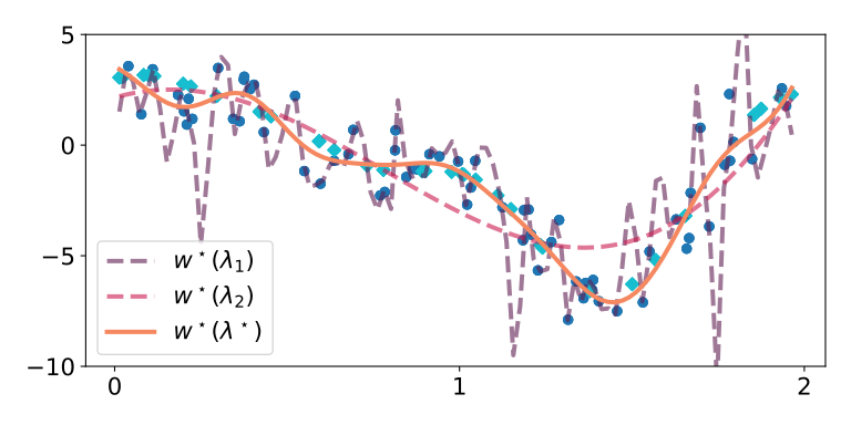
例如，这包括超参数优化：其中 $f$ 为内层的对数似然目标， $g$ 为外层的验证损失， ${\bm{w}}\in\mathcal{W}$ 为模型参数， ${\bm{\lambda}}\in\Lambda$ 则为模型超参数（如正则化强度），如图 11.1 所示。要最小化 $h({\bm{\lambda}})$ ，通常采用关于 ${\bm{\lambda}}$ 的梯度下降方案，这就需要对 $\nabla h({\bm{\lambda}})$ 进行计算。设 ${\bm{w}}^{\star}({\bm{\lambda}})$ 在 ${\bm{\lambda}}$ 处可微，则由链式法则可得雅可比矩阵This includes for instance hyperparameter optimization, where $f$ is an inner log-likelihood objective, $g$ is an outer validation loss, ${\bm{w}}\in\mathcal{W}$ are model parameters and ${\bm{\lambda}}\in\Lambda$ are model hyperparameters, such as regularization strength, as illustrated in Fig. 11.1. To minimize $h({\bm{\lambda}})$ , one generally resorts to a gradient descent scheme w.r.t. ${\bm{\lambda}}$ , which requires computing $\nabla h({\bm{\lambda}})$ . Assuming that ${\bm{w}}^{\star}({\bm{\lambda}})$ is differentiable at ${\bm{\lambda}}$ , by the chain rule, we obtain the Jacobian

\partial h({\bm{\lambda}})=\partial_{1}g({\bm{w}}^{\star}({\bm{\lambda}}),{\bm{\lambda}})\partial{\bm{w}}^{\star}({\bm{\lambda}})+\partial_{2}g({\bm{w}}^{\star}({\bm{\lambda}}),{\bm{\lambda}}).

借助 $\partial h({\bm{\lambda}})^{\top}=\nabla h({\bm{\lambda}})$ （见注 2.2.9），可得到梯度Using $\partial h({\bm{\lambda}})^{\top}=\nabla h({\bm{\lambda}})$ (see Remark 2.2.9), we obtain the gradient

\nabla h({\bm{\lambda}})=\partial{\bm{w}}^{\star}({\bm{\lambda}})^{\top}\nabla_{1}g({\bm{w}}^{\star}({\bm{\lambda}}),{\bm{\lambda}})+\nabla_{2}g({\bm{w}}^{\star}({\bm{\lambda}}),{\bm{\lambda}}).

唯一棘手的一项是 $\partial{\bm{w}}^{\star}({\bm{\lambda}})$ ，因为它涉及对 argmax 求导。事实上，大多数情况下 ${\bm{w}}^{\star}({\bm{\lambda}})$ 并无显式公式，也无法分解为初等函数。The only problematic term is $\partial{\bm{w}}^{\star}({\bm{\lambda}})$ , as it requires argmax differentiation. Indeed, most of the time, there is no explicit formula for ${\bm{w}}^{\star}({\bm{\lambda}})$ and it does not decompose into elementary functions.

图 11.1：非线性回归中的超参数优化可表述为双层优化问题。每条曲线对应以不同超参数

\lambda

拟合若干训练数据（蓝色圆点）所得的估计量。形式上，记

f

为训练目标，则估计量为

w^{\star}(\lambda)\coloneqq\argmin_{w}f(w;\lambda)

。目标是找到能最好地拟合若干验证数据（此处为青色菱形）的最优超参数，即最小化

h(\lambda)\coloneqq g(w^{\star}(\lambda),\lambda)

，其中

g

为验证目标。

\lambda_{1}

过小会导致对训练目标过拟合，在验证目标上表现不佳；反之，

\lambda_{2}

较大则会导致对训练目标和验证目标都欠拟合。最优参数

\lambda^{\star}

使验证目标最小，可通过对

\lambda

进行梯度下降迭代求得。这需要

h(\lambda)=g(w^{\star}(\lambda),\lambda)

关于

\lambda

的梯度。Figure 11.1: Hyperparameter optimization in nonlinear regression can be cast as a bi-level optimization problem. Each line corresponds to the estimator obtained by fitting some training data (in blue circles) using a different hyperparameter

\lambda

. Formally, denoting

f

the training objective, the estimators are

w^{\star}(\lambda)\coloneqq\argmin_{w}f(w;\lambda)

. The goal is to find the best hyperparameter that fits some validation data (here in cyan diamonds), that is, minimizing

h(\lambda)\coloneqq g(w^{\star}(\lambda),\lambda)

, where

g

is the validation objective. A too small

\lambda_{1}

leads to overfitting the training objective and performs badly on validation objective. Conversely, a larger

\lambda_{2}

underfits both training and validation objectives. The optimal parameter

\lambda^{\star}

minimizes the validation objective and may be obtained by iterating gradient descent w.r.t.

\lambda

. This requires gradients of

h(\lambda)=g(w^{\star}(\lambda),\lambda)

w.r.t.

\lambda

.

11.2 包络定理11.2 Envelope theorems

在 $g=f$ 这一特殊情形下，式 11.1 所定义的复合 $h$ 简化为In the special case $g=f$ , the composition $h$ defined in Eq. 11.1 is simply given by

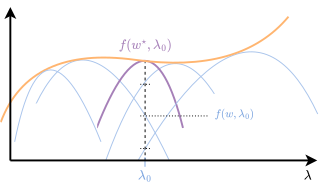
h({\bm{\lambda}})=f({\bm{w}}^{\star}({\bm{\lambda}}),{\bm{\lambda}})=\max_{{\bm{w}}\in\mathcal{W}}f({\bm{w}},{\bm{\lambda}}).

也就是说，此时不再需要对 argmax 求导，而只需对 max 求导；下文将会看到，后者要容易得多。函数 $h$ 常被称为值函数 [66]。“包络”这一名称的由来如图 11.2 所示。需要强调，包络定理并非只有一条，而是有多条，具体取决于对 $f$ 所作的假设。That is, we no longer need argmax differentiation, but only max differentiation, which, as we shall now see is much easier. The function $h$ is often called a value function [66]. The reason for the name “envelope” is illustrated in Fig. 11.2. We emphasize that there is not one, but several envelope theorems, depending on the assumptions on $f$ .

图 11.2：

h({\bm{\lambda}})=\max_{{\bm{w}}\in\mathcal{W}}f({\bm{w}},{\bm{\lambda}})

的图像是所有

{\bm{w}}\in\mathcal{W}

对应的函数

{\bm{\lambda}}\mapsto f({\bm{w}},{\bm{\lambda}})

的图像的上包络。Figure 11.2: The graph of

h({\bm{\lambda}})=\max_{{\bm{w}}\in\mathcal{W}}f({\bm{w}},{\bm{\lambda}})

is the upper-envelope of the graphs of the functions

{\bm{\lambda}}\mapsto f({\bm{w}},{\bm{\lambda}})

for all

{\bm{w}}\in\mathcal{W}

.

11.2.1 Bertsekas 定理Bertsekas’ theorem

以下定理取自 [24, 命题 B.25]。The following theorem is due to [24, Proposition B.25].

定理 11.2.1（Bertsekas 定理）。Theorem 11.2.1 (Bertsekas’ theorem).

令Let

h({\bm{\lambda}})\coloneqq\max_{{\bm{w}}\in\mathcal{W}}f({\bm{w}},{\bm{\lambda}})

以及and

{\bm{w}}^{\star}({\bm{\lambda}})\coloneqq\argmax_{{\bm{w}}\in\mathcal{W}}f({\bm{w}},{\bm{\lambda}}),

其中

f\colon\mathcal{W}\times\Lambda\to\mathbb{R}

关于

{\bm{w}}

是凹的，且

\mathcal{W}

是一个紧凸集。若最大值

{\bm{w}}^{\star}({\bm{\lambda}})

唯一，则函数

h

可微，其梯度为where

f\colon\mathcal{W}\times\Lambda\to\mathbb{R}

is concave in

{\bm{w}}

and

\mathcal{W}

is a compact convex set. If the maximum

{\bm{w}}^{\star}({\bm{\lambda}})

is unique, then the function

h

is differentiable with gradient

\nabla h({\bm{\lambda}})=\nabla_{2}f({\bm{w}}^{\star}({\bm{\lambda}}),{\bm{\lambda}}).

若进一步

f

关于

{\bm{\lambda}}

是凸的，则

h({\bm{\lambda}})

是凸的。If furthermore

f

is convex in

{\bm{\lambda}}

, then

h({\bm{\lambda}})

is convex.

当 $\mathcal{W}=\mathbb{R}^{P}$ 时，可以给出该定理的一个变体。A variant of the theorem can be stated when $\mathcal{W}=\mathbb{R}^{P}$ .

定理 11.2.2（无界情形）。Theorem 11.2.2 (Unbounded case).

假设

\mathcal{W}=\mathbb{R}^{P}

。若

f

关于

{\bm{w}}

是强凹的，则函数

h

可微，其梯度为Suppose

\mathcal{W}=\mathbb{R}^{P}

. If

f

is strongly concave in

{\bm{w}}

, then the function

h

is differentiable with gradient

\nabla h({\bm{\lambda}})=\nabla_{2}f({\bm{w}}^{\star}({\bm{\lambda}}),{\bm{\lambda}}).

若进一步

f

关于

{\bm{\lambda}}

是凸的，则

h({\bm{\lambda}})

也是凸的。If furthermore

f

is convex in

{\bm{\lambda}}

, then

h({\bm{\lambda}})

is convex.

直观地说，定理 11.2.1 与定理 11.2.2 意味着我们可以把 ${\bm{w}}^{\star}({\bm{\lambda}})$ 当作 ${\bm{\lambda}}$ 的一个常数来处理。换言之，我们不需要穿过 ${\bm{w}}^{\star}({\bm{\lambda}})$ 进行求导，即使它依赖于 ${\bm{\lambda}}$ 。Informally, Theorem 11.2.1 and Theorem 11.2.2 mean that we can treat ${\bm{w}}^{\star}({\bm{\lambda}})$ as if it were a constant of ${\bm{\lambda}}$ . In other words, we do not need to differentiate through ${\bm{w}}^{\star}({\bm{\lambda}})$ , even though it depends on ${\bm{\lambda}}$ .

注 11.2.3（历史注记）。Remark 11.2.3 (Historical note).

在机器学习文献中，Bertsekas 定理或其无界变体常被误引作 Danskin 定理，因为 Bertsekas 本人正是这样称呼它的 [24, Proposition B.25]。然而，两者的假设并不相同，因此更应将其视为 Danskin 原始定理的变体或推论。详见第 11.2.3 节。Bertsekas’ theorem or its unbounded variant are often incorrectly cited as Danskin’s theorem in the machine learning literature, because Bertsekas himself called it that way [24, Proposition B.25]. However, because the assumptions differ, they should rather be thought as variants or corollaries of Danskin’s original theorem. See Section 11.2.3 for more details.

现在，我们借助定理 11.2.2 说明如何穿过最小值 $h({\bm{\lambda}})=\min_{{\bm{w}}\in\mathcal{W}}f({\bm{w}},{\bm{\lambda}})$ 进行求导，其中假定 $f({\bm{w}},{\bm{\lambda}})$ 关于 ${\bm{w}}$ 是强凸的。We now illustrate Theorem 11.2.2, to differentiate through a minimum, $h({\bm{\lambda}})=\min_{{\bm{w}}\in\mathcal{W}}f({\bm{w}},{\bm{\lambda}})$ , assuming $f({\bm{w}},{\bm{\lambda}})$ is strongly convex in ${\bm{w}}$ .

例 11.2.4（对凸二次函数的最小值求导）。Example 11.2.4 (Differentiating the minimum of a convex quadratic).

令

h(\lambda)\coloneqq\min_{w\in\mathbb{R}}f(w,\lambda)

，其中

f(w,\lambda)\coloneqq\frac{\lambda}{2}w^{2}+bw+c

，

\lambda>0

。

f

关于

w

的导数为

\nabla_{1}f(w,\lambda)=\lambda w+b

；

f

关于

w

的二阶导数为

\nabla_{1}^{2}f(w,\lambda)=\lambda

。因此，

f

关于

w

是强凸的。设

w^{\star}(\lambda)

为

f

在

w

上的最小值。令

\nabla_{1}f(w,\lambda)

等于零，可得

w^{\star}(\lambda)=-\frac{b}{\lambda}

。

f

关于

\lambda

的导数为

\nabla_{2}f(w,\lambda)=\frac{1}{2}w^{2}

。由定理 11.2.2 可得

h^{\prime}(\lambda)=\nabla_{2}f(w^{\star}(\lambda),\lambda)=\frac{1}{2}(w^{\star}(\lambda))^{2}=\frac{1}{2}\frac{b^{2}}{\lambda^{2}}

。下面验证该导数确实无误：将

w^{\star}(\lambda)

代回

f(w,\lambda)

，即得解析公式

h(\lambda)=-\frac{1}{2}\frac{b^{2}}{\lambda}+c

。利用

(\frac{1}{\lambda})^{\prime}=-\frac{1}{\lambda^{2}}

，我们确实得到了

h^{\prime}(\lambda)

的同一表达式。Let us define

h(\lambda)\coloneqq\min_{w\in\mathbb{R}}f(w,\lambda)

, where

f(w,\lambda)\coloneqq\frac{\lambda}{2}w^{2}+bw+c

and

\lambda>0

. The derivative of

f

w.r.t.

w

is

\nabla_{1}f(w,\lambda)=\lambda w+b

. The second derivative of

f

w.r.t.

w

is

\nabla_{1}^{2}f(w,\lambda)=\lambda

. Therefore

f

is strongly convex in

w

. Let

w^{\star}(\lambda)

be the minimum of

f

in

w

. Setting

\nabla_{1}f(w,\lambda)

to zero, we get

w^{\star}(\lambda)=-\frac{b}{\lambda}

. The derivative of

f

w.r.t.

\lambda

is

\nabla_{2}f(w,\lambda)=\frac{1}{2}w^{2}

. From Theorem 11.2.2, we have

h^{\prime}(\lambda)=\nabla_{2}f(w^{\star}(\lambda),\lambda)=\frac{1}{2}(w^{\star}(\lambda))^{2}=\frac{1}{2}\frac{b^{2}}{\lambda^{2}}

. Let us check that the derivative is indeed correct. Plugging

w^{\star}(\lambda)

back into

f(w,\lambda)

, we get the analytical formula

h(\lambda)=-\frac{1}{2}\frac{b^{2}}{\lambda}+c

. Using

(\frac{1}{\lambda})^{\prime}=-\frac{1}{\lambda^{2}}

, we indeed obtain the same expression for

h^{\prime}(\lambda)

.

如下所示，对于关于 ${\bm{\lambda}}$ 为仿射的函数，定理 11.2.1 有一个简单的解释。Theorem 11.2.1 has a simple interpretation for functions that are affine in ${\bm{\lambda}}$ as shown below.

例 11.2.5（凸共轭）。Example 11.2.5 (Convex conjugate).

设

f({\bm{w}},{\bm{\lambda}})\coloneqq\langle{\bm{w}},{\bm{\lambda}}\rangle-\Omega({\bm{w}})

，其中

\Omega

为凸。于是有

h({\bm{\lambda}})=\max_{{\bm{w}}\in\mathcal{W}} \ \langle{\bm{w}},{\bm{\lambda}}\rangle-\Omega({\bm{w}})\eqqcolon\Omega^{*}({\bm{\lambda}})

，其中

\Omega^{*}

表示

\Omega

的凸共轭。由于

f

是凸的，且假设

\mathcal{W}

为凸紧集，定理 11.2.1 的条件得以满足。由

\nabla_{2}f({\bm{w}},{\bm{\lambda}})={\bm{w}}

可得

\nabla h({\bm{\lambda}})=\nabla\Omega^{*}({\bm{\lambda}})={\bm{w}}^{\star}({\bm{\lambda}})

。换言之，在这一特殊情形下，最大值的梯度等于 argmax。其原因在于

f({\bm{w}},{\bm{\lambda}})

关于

{\bm{\lambda}}

是仿射的。Let

f({\bm{w}},{\bm{\lambda}})\coloneqq\langle{\bm{w}},{\bm{\lambda}}\rangle-\Omega({\bm{w}})

with

\Omega

convex. We then have

h({\bm{\lambda}})=\max_{{\bm{w}}\in\mathcal{W}} \ \langle{\bm{w}},{\bm{\lambda}}\rangle-\Omega({\bm{w}})\eqqcolon\Omega^{*}({\bm{\lambda}})

, where

\Omega^{*}

denotes the convex conjugate of

\Omega

. Since

f

is convex and assuming

\mathcal{W}

is convex compact, the conditions of Theorem 11.2.1 are met. Since

\nabla_{2}f({\bm{w}},{\bm{\lambda}})={\bm{w}}

, we obtain

\nabla h({\bm{\lambda}})=\nabla\Omega^{*}({\bm{\lambda}})={\bm{w}}^{\star}({\bm{\lambda}})

. In other words, in this special case, the gradient of the max is equal to the argmax. This is due to the fact that

f({\bm{w}},{\bm{\lambda}})

is affine in

{\bm{\lambda}}

.

另一个应用是鞍点优化。Another application is saddle point optimization.

例 11.2.6（鞍点问题）。Example 11.2.6 (Saddle point problem).

考虑鞍点问题

\min_{{\bm{\lambda}}\in\Lambda}\max_{{\bm{w}}\in\mathcal{W}}f({\bm{w}},{\bm{\lambda}})

。若关于

{\bm{\lambda}}

求最小较为困难，而关于

{\bm{w}}

求最大较为容易，我们便可把问题改写为

\min_{{\bm{\lambda}}\in\Lambda}h({\bm{\lambda}})

，其中

h({\bm{\lambda}})\coloneqq\max_{{\bm{w}}\in\mathcal{W}}f({\bm{w}},{\bm{\lambda}})

，并借助

\nabla h({\bm{\lambda}})

关于

{\bm{\lambda}}

执行（投影）梯度下降。Consider the saddle point problem

\min_{{\bm{\lambda}}\in\Lambda}\max_{{\bm{w}}\in\mathcal{W}}f({\bm{w}},{\bm{\lambda}})

. If it is difficult to minimize w.r.t.

{\bm{\lambda}}

but easy to maximize w.r.t.

{\bm{w}}

, we can rewrite the problem as

\min_{{\bm{\lambda}}\in\Lambda}h({\bm{\lambda}})

, where

h({\bm{\lambda}})\coloneqq\max_{{\bm{w}}\in\mathcal{W}}f({\bm{w}},{\bm{\lambda}})

, and use

\nabla h({\bm{\lambda}})

to perform (projected) gradient descent w.r.t.

{\bm{\lambda}}

.

11.2.2 Rockafellar 定理Rockafellar’s theorem

在与 $f$ 相关的不同假设下，可以证明一个相关定理 [169, 定理 10.31]。A related theorem [169, Theorem 10.31] can be proved under different assumptions on $f$ .

定理 11.2.7（Rockafellar 包络定理）。Theorem 11.2.7 (Rockafellar’s envelope theorem).

设

f\colon\mathcal{W}\times\Lambda\to\mathbb{R}

，并设

\mathcal{W}

为紧凸集。令Let

f\colon\mathcal{W}\times\Lambda\to\mathbb{R}

and

\mathcal{W}

be a compact convex set. Let

h({\bm{\lambda}})\coloneqq\max_{{\bm{w}}\in\mathcal{W}}f({\bm{w}},{\bm{\lambda}})

以及and

{\bm{w}}^{\star}({\bm{\lambda}})\coloneqq\argmax_{{\bm{w}}\in\mathcal{W}}f({\bm{w}},{\bm{\lambda}}).

若对任意

{\bm{w}}\in\mathcal{W}

，

f

都在

{\bm{\lambda}}

上连续可微，

\nabla_{1}f

连续，且最大值

{\bm{w}}^{\star}({\bm{\lambda}})

唯一，则函数

h

可微，其梯度为If

f

is continuously differentiable in

{\bm{\lambda}}

for all

{\bm{w}}\in\mathcal{W}

,

\nabla_{1}f

is continuous and the maximum

{\bm{w}}^{\star}({\bm{\lambda}})

is unique, then the function

h

is differentiable with gradient

\nabla h({\bm{\lambda}})=\nabla_{2}f({\bm{w}}^{\star}({\bm{\lambda}}),{\bm{\lambda}}).

与 Bertsekas 定理相比，Rockafellar 定理不要求 $f$ 关于 ${\bm{w}}$ 为凹，但对 $f$ 的可微性提出了更强的假设。Compared to Bertsekas’ theorem, Rockafellar’s theorem does not require $f$ to be concave in ${\bm{w}}$ , but it requires stronger assumptions on the differentiability of $f$ .

11.2.3 Danskin 定理Danskin’s theorem

最后，我们陈述 Danskin 的原始定理 [51]。Finally, we state Danskin’s original theorem [51].

定理 11.2.8（Danskin 定理）。Theorem 11.2.8 (Danskin’s theorem).

设

\mathcal{W}

为一个紧拓扑空间。设

f\colon\mathcal{W}\times\Lambda\to\mathbb{R}

连续，且关于

{\bm{\lambda}}\in\Lambda

连续可微。将值函数与最大值点集分别定义为Let

\mathcal{W}

be a compact topological space. Let

f\colon\mathcal{W}\times\Lambda\to\mathbb{R}

be continuous and continuously differentiable with respect to

{\bm{\lambda}}\in\Lambda

. Let the value function and the set of maximizers be defined as

h({\bm{\lambda}})\coloneqq\max_{{\bm{w}}\in\mathcal{W}}f({\bm{w}},{\bm{\lambda}})\quad\text{and}\quad\mathcal{W}^{\star}({\bm{\lambda}})\coloneqq\argmax_{{\bm{w}}\in\mathcal{W}}f({\bm{w}},{\bm{\lambda}}).

则

h

在

{\bm{\lambda}}\in\Lambda

处沿方向

{\bm{d}}\in\Lambda

的方向导数（记作

h^{\prime}({\bm{\lambda}};{\bm{d}})

）存在，且由下式给出：Then, the directional derivative of

h

at

{\bm{\lambda}}\in\Lambda

in direction

{\bm{d}}\in\Lambda

, denoted

h^{\prime}({\bm{\lambda}};{\bm{d}})

, exists and is given by

h^{\prime}({\bm{\lambda}};{\bm{d}})=\max_{{\bm{w}}\in\mathcal{W}^{\star}({\bm{\lambda}})}\langle\nabla_{2}f({\bm{w}},{\bm{\lambda}}),{\bm{d}}\rangle.

我们在表 11.1 中总结各包络定理及其假设。We sum up envelope theorems and their assumptions in Table 11.1.

表 11.1：不同包络定理的比较。Table 11.1: Comparison of different envelope theorems.

定理Theorem	${\bm{w}}^{\star}$ 是否唯一？Unique ${\bm{w}}^{\star}$ ?	关于 ${\bm{w}}$ 是否为凹？Concave in ${\bm{w}}$ ?	关于 ${\bm{w}}$ 是否光滑？Smooth in ${\bm{w}}$ ?	结果Result
DanskinDanskin	否No	否No	否No	方向导数Dir. Deriv.
BertsekasBertsekas	是Yes	是Yes	否No	梯度Gradient
RockafellarRockafellar	是Yes	否No	是Yes	梯度Gradient

11.3 隐函数定理11.3 Implicit function theorem

11.3.1 一元函数Univariate functions

隐函数定理（IFT）给出了如下条件：在该条件下，形如 $F(w,\lambda)=0$ 的隐式关系可以在局部改写为函数 $w=w^{\star}(\lambda)$ ，并给出一种计算其关于 $\lambda$ 的导数的方法。The implicit function theorem (IFT) provides conditions under which an implicit relationship of the form $F(w,\lambda)=0$ can be rewritten as a function $w=w^{\star}(\lambda)$ locally, and provides a way to compute its derivative w.r.t. $\lambda$ .

定理 11.3.1（隐函数定理，一元情形）。Theorem 11.3.1 (Implicit function theorem, univariate case).

设

F\colon\mathbb{R}\times\mathbb{R}\to\mathbb{R}

。假设

F(w,\lambda)

是

(w_{0},\lambda_{0})

的某邻域

\mathcal{U}

内的连续可微函数，且满足

F(w_{0},\lambda_{0})=0

与

\partial_{1}F(w_{0},\lambda_{0})\neq 0

。则存在

(w_{0},\lambda_{0})

的一个邻域

\mathcal{V}\subseteq\mathcal{U}

，其中存在函数

w^{\star}(\lambda)

，使得Let

F\colon\mathbb{R}\times\mathbb{R}\to\mathbb{R}

. Assume

F(w,\lambda)

is a continuously differentiable function in a neighborhood

\mathcal{U}

of

(w_{0},\lambda_{0})

such that

F(w_{0},\lambda_{0})=0

and

\partial_{1}F(w_{0},\lambda_{0})\neq 0

. Then there exists a neighborhood

\mathcal{V}\subseteq\mathcal{U}

of

(w_{0},\lambda_{0})

in which there is a function

w^{\star}(\lambda)

such that •

w^{\star}(\lambda_{0})=w_{0}

, • 对邻域

\mathcal{V}

内的任意

\lambda

，均有

F(w^{\star}(\lambda),\lambda)=0

，

F(w^{\star}(\lambda),\lambda)=0

for all

\lambda

in the neighborhood

\mathcal{V}

, •

\partial w^{\star}(\lambda)=-\frac{\partial_{2}F(w^{\star}(\lambda),\lambda)}{\partial_{1}F(w^{\star}(\lambda),\lambda)}

.

我们将证明推迟到多元情形，先从一个经典的应用该定理的例子开始。We postpone the proof to the multivariate case and begin with a classical example of application of the theorem.

图 11.3：圆的方程

F(x,y)\coloneqq x^{2}+y^{2}-1=0

并不是从

y\in[-1,1]

到

x\in[-1,1]

的函数，因为总有两个可能的

x

取值，即

x=\sqrt{1-y^{2}}

或

x=-\sqrt{1-y^{2}}

。然而，在某点

(x_{0},y_{0})

的局部邻域内，例如满足

x_{0}>0

和

y_{0}>0

（右上象限）时，函数

x=x^{\star}(y)=\sqrt{1-y^{2}}

是良定义的。隐函数定理给出了这样的函数在局部存在的条件，并提供了一种计算其导数的方法。Figure 11.3: The circle equation

F(x,y)\coloneqq x^{2}+y^{2}-1=0

is not a function from

y\in[-1,1]

to

x\in[-1,1]

, as there are always two possible

x

values,

x=\sqrt{1-y^{2}}

or

x=-\sqrt{1-y^{2}}

. However, locally around some point

(x_{0},y_{0})

, e.g., such that

x_{0}>0

and

y_{0}>0

(upper-right quadrant), the function

x=x^{\star}(y)=\sqrt{1-y^{2}}

is well-defined. The implicit function theorem gives conditions for such a function to exist locally and provides a way to compute its derivative.

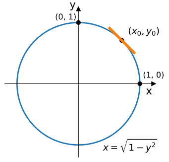
例 11.3.2（单位圆的方程）。Example 11.3.2 (Equation of the unit circle).

为清晰起见，我们使用

w\equiv x

与

\lambda\equiv y

。设

F(x,y)\coloneqq x^{2}+y^{2}-1

。一般而言，我们无法把单位圆方程

F(x,y)=0

改写为从

y

到

x

的函数，因为对每个

y\in[-1,1]

，总有两个可能的

x

值，即

x=\sqrt{1-y^{2}}

或

x=-\sqrt{1-y^{2}}

。但在某一点

(x_{0},y_{0})

的局部附近，例如在满足

x_{0}>0

与

y_{0}>0

时（右上象限），函数

x=x^{\star}(y)=\sqrt{1-y^{2}}

有良定义。借助

\partial_{1}F(x,y)=2x

与

\partial_{2}F(x,y)=2y

，我们在该邻域内（此例中即右上象限）得到

\partial x^{\star}(y)=-\frac{\partial_{2}F(x^{\star}(y),y)}{\partial_{1}F(x^{\star}(y),y)}=-\frac{2y}{2x^{\star}(y)}=-\frac{y}{\sqrt{1-y^{2}}}

。这与对

\sqrt{1-y^{2}}

施用链式法则所得的导数表达式完全相同，且在

y\in[0,1)

上有良定义。We use

w\equiv x

and

\lambda\equiv y

for clarity. Let

F(x,y)\coloneqq x^{2}+y^{2}-1

. In general, we cannot rewrite the unit circle equation

F(x,y)=0

as a function from

y

to

x

, because for every

y\in[-1,1]

, there are always two possible

x

values, namely,

x=\sqrt{1-y^{2}}

or

x=-\sqrt{1-y^{2}}

. However, locally around some point

(x_{0},y_{0})

, e.g., such that

x_{0}>0

and

y_{0}>0

(upper-right quadrant), the function

x=x^{\star}(y)=\sqrt{1-y^{2}}

is well-defined. Using

\partial_{1}F(x,y)=2x

and

\partial_{2}F(x,y)=2y

, we get

\partial x^{\star}(y)=-\frac{\partial_{2}F(x^{\star}(y),y)}{\partial_{1}F(x^{\star}(y),y)}=-\frac{2y}{2x^{\star}(y)}=-\frac{y}{\sqrt{1-y^{2}}}

in that neighborhood (the upper right quadrant in this case). This is indeed the same derivative expression as if we used the chain rule on

\sqrt{1-y^{2}}

and is well-defined on

y\in[0,1)

.

在上述简单例子中，我们可以容易地在给定邻域内推导出联系 $y$ 与 $x$ 的显式函数，但这并非总是可行。隐函数定理给出了保证这样的函数存在的条件以及对其求导的方法，但并不给出构造该函数的方法。事实上，寻找使 $F(w^{\star}(\lambda),\lambda)=0$ 成立的 $w^{\star}(\lambda)$ ，通常涉及求根算法、优化算法、非线性系统求解器等。In the above simple example, we can easily derive an explicit function relating $y$ to $x$ in a given neighborhood, but this is not always the case. The IFT gives us conditions guaranteeing that such function exists and a way to differentiate it, but not a way to construct such a function. In fact, finding $w^{\star}(\lambda)$ such that $F(w^{\star}(\lambda),\lambda)=0$ typically involves a root finding algorithm, an optimization algorithm, a nonlinear system solver, etc.

例 11.3.3（多项式）。Example 11.3.3 (Polynomial).

设

F(w,\lambda)=w^{5}+w^{3}+w-\lambda

。根据 Abel-Ruffini 定理 [196]，五次多项式（次数为

5

的多项式）的根不能用根式表示，只能借助数值求根。此外，奇次多项式必有实根；并且

\partial_{1}F(w,\lambda)=5w^{4}+3w^{2}+1

严格为正。因此由介值定理，满足

F(w^{\star}(\lambda),\lambda)=0

的根

w^{\star}(\lambda)

必定唯一。这个唯一根例如可用二分法求得。利用 IFT 可得其导数为

\partial w^{\star}(\lambda)=(5w^{\star}(\lambda)^{4}+3w^{\star}(\lambda)^{2}+1)^{-1}

。Let

F(w,\lambda)=w^{5}+w^{3}+w-\lambda

. According to the Abel-Ruffini theorem [196], quintics (polynomials of degree

5

) do not enjoy roots in terms of radicals and one must resort to numerical root finding. In addition, odd-degree polynomials have real roots. Moreover,

\partial_{1}F(w,\lambda)=5w^{4}+3w^{2}+1

is strictly positive. Therefore, by the intermediate value theorem, there must be only one root

w^{\star}(\lambda)

such that

F(w^{\star}(\lambda),\lambda)=0

. This unique root can for example be found by bisection. Using the IFT, its derivative is found to be

\partial w^{\star}(\lambda)=(5w^{\star}(\lambda)^{4}+3w^{\star}(\lambda)^{2}+1)^{-1}

.

若 IFT 的假设在某点的邻域内成立，则隐函数在该点可微；但反之不成立：IFT 假设不成立并不必然意味着隐函数不可微，下面我们对此加以说明。While an implicit function is differentiable at a point if the assumptions of the IFT hold in a neighborhood of that point, the reciprocal is not true: failure of the IFT assumptions does not necessarily mean that the implicit function is not differentiable, as we now illustrate.

例 11.3.4（隐函数定理的条件并非可微性的必要条件）。Example 11.3.4 (IFT conditions are not necessary for differentiability).

考虑

F(w,\lambda)=(w-\lambda)^{2}

。若将

w^{\star}(\lambda)=\lambda

定义为恒等函数，则显然有

F(w^{\star}(\lambda),\lambda)=0

。它对所有

\lambda

显然可微，但 IFT 的假设却不成立，因为我们有

\partial_{1}F(w,\lambda)=2(w-\lambda)

，从而

\partial_{1}F(0,0)=0

。Consider

F(w,\lambda)=(w-\lambda)^{2}

. We clearly have that

F(w^{\star}(\lambda),\lambda)=0

if we define

w^{\star}(\lambda)=\lambda

, the identity function. It is clearly differentiable for all

\lambda

, yet the assumptions of the IFT fail, since we have

\partial_{1}F(w,\lambda)=2(w-\lambda)

and therefore

\partial_{1}F(0,0)=0

.

11.3.2 多元函数Multivariate functions

现在我们给出一般多元情形下的隐函数定理。非正式地说，若 $F({\bm{w}}^{\star}({\bm{\lambda}}),{\bm{\lambda}})={\mathbf{0}}$ ，则由链式法则，我们有We now present the IFT in the general multivariate setting. Informally, if $F({\bm{w}}^{\star}({\bm{\lambda}}),{\bm{\lambda}})={\mathbf{0}}$ , then by the chain rule, we have

\partial_{1}F({\bm{w}}^{\star}({\bm{\lambda}}),{\bm{\lambda}})\partial{\bm{w}}^{\star}({\bm{\lambda}})+\partial_{2}F({\bm{w}}^{\star}({\bm{\lambda}}),{\bm{\lambda}})={\mathbf{0}},

这意味着雅可比矩阵 $\partial{\bm{w}}^{\star}({\bm{\lambda}})$ （假设存在）满足meaning that the Jacobian $\partial{\bm{w}}^{\star}({\bm{\lambda}})$ , assuming that it exists, satisfies

-\partial_{1}F({\bm{w}}^{\star}({\bm{\lambda}}),{\bm{\lambda}})\partial{\bm{w}}^{\star}({\bm{\lambda}})=\partial_{2}F({\bm{w}}^{\star}({\bm{\lambda}}),{\bm{\lambda}}).

隐函数定理给出了 $\partial{\bm{w}}^{\star}({\bm{\lambda}})$ 存在的条件。The IFT gives us conditions for the existence of $\partial{\bm{w}}^{\star}({\bm{\lambda}})$ .

定理 11.3.5（隐函数定理，多元情形）。Theorem 11.3.5 (Implicit function theorem, multivariate case).

我们定义

F\colon\mathcal{W}\times\Lambda\to\mathcal{W}

。设

F({\bm{w}},{\bm{\lambda}})

是

({\bm{w}}_{0},{\bm{\lambda}}_{0})

的某邻域内的连续可微函数，满足

F({\bm{w}}_{0},{\bm{\lambda}}_{0})={\mathbf{0}}

，且

\partial_{1}F({\bm{w}}_{0},{\bm{\lambda}}_{0})

可逆，即其行列式非零。则存在

{\bm{\lambda}}_{0}

的一个邻域，其中存在函数

{\bm{w}}^{\star}({\bm{\lambda}})

，使得Let us define

F\colon\mathcal{W}\times\Lambda\to\mathcal{W}

. Assume

F({\bm{w}},{\bm{\lambda}})

is a continuously differentiable function in a neighborhood of

({\bm{w}}_{0},{\bm{\lambda}}_{0})

such that

F({\bm{w}}_{0},{\bm{\lambda}}_{0})={\mathbf{0}}

and

\partial_{1}F({\bm{w}}_{0},{\bm{\lambda}}_{0})

is invertible, i.e., its determinant is nonzero. Then there exists a neighborhood of

{\bm{\lambda}}_{0}

in which there is a function

{\bm{w}}^{\star}({\bm{\lambda}})

such that •

{\bm{w}}^{\star}({\bm{\lambda}}_{0})={\bm{w}}_{0}

, • 对邻域内的所有

{\bm{\lambda}}

，均有

F({\bm{w}}^{\star}({\bm{\lambda}}),{\bm{\lambda}})={\mathbf{0}}

，

F({\bm{w}}^{\star}({\bm{\lambda}}),{\bm{\lambda}})={\mathbf{0}}

for all

{\bm{\lambda}}

in the neighborhood, •

-\partial_{1}F({\bm{w}}^{\star}({\bm{\lambda}}),{\bm{\lambda}})\partial{\bm{w}}^{\star}({\bm{\lambda}})=\partial_{2}F({\bm{w}}^{\star}({\bm{\lambda}}),{\bm{\lambda}})

\iff\partial{\bm{w}}^{\star}({\bm{\lambda}})=-\partial_{1}F({\bm{w}}^{\star}({\bm{\lambda}}),{\bm{\lambda}})^{-1}\partial_{2}F({\bm{w}}^{\star}({\bm{\lambda}}),{\bm{\lambda}}).

我们从一个简单的无约束优化算法开始。We begin with a simple unconstrained optimization algorithm.

例 11.3.6（无约束优化）。Example 11.3.6 (Unconstrained optimization).

假设我们希望穿过

{\bm{w}}^{\star}({\bm{\lambda}})=\argmin_{{\bm{w}}\in\mathbb{R}^{P}}f({\bm{w}},{\bm{\lambda}})

求导，其中

f

关于

{\bm{w}}

严格凸，从而保证解唯一。由驻值条件，若定义

F({\bm{w}},{\bm{\lambda}})\coloneqq\nabla_{1}f({\bm{w}},{\bm{\lambda}})

，则

{\bm{w}}^{\star}({\bm{\lambda}})

可唯一地刻画为

F

在第一个自变量上的根，即

F({\bm{w}}^{\star}({\bm{\lambda}}),{\bm{\lambda}})={\mathbf{0}}

。式中

\partial_{1}F({\bm{w}},{\bm{\lambda}})=\nabla^{2}_{1}f({\bm{w}},{\bm{\lambda}})

是

f

关于

{\bm{w}}

的 Hessian 矩阵，

\partial_{2}F({\bm{w}},{\bm{\lambda}})=\partial_{2}\nabla_{1}f({\bm{w}},{\bm{\lambda}})

则是

f

关于

{\bm{w}}

与

{\bm{\lambda}}

的交叉导数。因此，只要 Hessian 矩阵在

({\bm{w}}^{\star}({\bm{\lambda}}),{\bm{\lambda}})

处有良定义且可逆，我们便可利用 IFT 穿过

{\bm{w}}^{\star}({\bm{\lambda}})

求导，得到

\partial{\bm{w}}^{\star}({\bm{\lambda}})=-(\nabla^{2}_{1}f({\bm{w}}^{\star}({\bm{\lambda}}),{\bm{\lambda}}))^{-1}\partial_{2}\nabla_{1}f({\bm{w}}^{\star}({\bm{\lambda}}),{\bm{\lambda}})

。Assume we want to differentiate through

{\bm{w}}^{\star}({\bm{\lambda}})=\argmin_{{\bm{w}}\in\mathbb{R}^{P}}f({\bm{w}},{\bm{\lambda}})

, where

f

is strictly convex in

{\bm{w}}

, which ensures that the solution is unique. From the stationary conditions, if we define

F({\bm{w}},{\bm{\lambda}})\coloneqq\nabla_{1}f({\bm{w}},{\bm{\lambda}})

, then

{\bm{w}}^{\star}({\bm{\lambda}})

is uniquely characterized as the root of

F

in the first argument, i.e.,

F({\bm{w}}^{\star}({\bm{\lambda}}),{\bm{\lambda}})={\mathbf{0}}

. We have

\partial_{1}F({\bm{w}},{\bm{\lambda}})=\nabla^{2}_{1}f({\bm{w}},{\bm{\lambda}})

, the Hessian of

f

in

{\bm{w}}

, and

\partial_{2}F({\bm{w}},{\bm{\lambda}})=\partial_{2}\nabla_{1}f({\bm{w}},{\bm{\lambda}})

, the cross derivatives of

f

in

{\bm{w}}

and

{\bm{\lambda}}

. Therefore, assuming that the Hessian is well-defined and invertible at

({\bm{w}}^{\star}({\bm{\lambda}}),{\bm{\lambda}})

, we can use the IFT to differentiate through

{\bm{w}}^{\star}({\bm{\lambda}})

and obtain

\partial{\bm{w}}^{\star}({\bm{\lambda}})=-(\nabla^{2}_{1}f({\bm{w}}^{\star}({\bm{\lambda}}),{\bm{\lambda}}))^{-1}\partial_{2}\nabla_{1}f({\bm{w}}^{\star}({\bm{\lambda}}),{\bm{\lambda}})

.

接下来，我们通过允许优化问题带有约束来推广前一例子。Next, we generalize the previous example, by allowing constraints in the optimization problem.

例 11.3.7（约束优化）。Example 11.3.7 (Constrained optimization).

现在假设我们希望穿过

{\bm{w}}^{\star}({\bm{\lambda}})=\argmin_{{\bm{w}}\in\mathcal{C}}f({\bm{w}},{\bm{\lambda}})

求导，其中

f

关于

{\bm{w}}

严格凸，且

\mathcal{C}\subseteq\mathcal{W}

为凸集。此时解由不动点方程

{\bm{w}}^{\star}({\bm{\lambda}})=P_{\mathcal{C}}({\bm{w}}^{\star}({\bm{\lambda}})-\eta\nabla_{1}f({\bm{w}}^{\star}({\bm{\lambda}}),{\bm{\lambda}}))

刻画：对任意

\eta>0

，

P({\bm{y}})\coloneqq\argmin_{{\bm{x}}\in\mathcal{C}}\|{\bm{x}}-{\bm{y}}\|_{2}^{2}

是

{\bm{y}}

到

\mathcal{C}

的欧几里得投影。因此，

{\bm{w}}^{\star}({\bm{\lambda}})

是

F({\bm{w}},{\bm{\lambda}})={\bm{w}}-P_{\mathcal{C}}({\bm{w}}-\eta\nabla_{1}f({\bm{w}},{\bm{\lambda}}))

的根（见第 16 章）。在定理条件成立的前提下，我们可以利用 IFT 穿过

{\bm{w}}^{\star}({\bm{\lambda}})

求导。注意，

\partial_{1}F({\bm{w}},{\bm{\lambda}})

需要给出雅可比矩阵

\partial P_{\mathcal{C}}({\bm{y}})

的表达式。所幸对许多集合

\mathcal{C}

而言，

P_{\mathcal{C}}({\bm{y}})

及其雅可比矩阵都易于计算 [27]。Now, assume we want to differentiate through

{\bm{w}}^{\star}({\bm{\lambda}})=\argmin_{{\bm{w}}\in\mathcal{C}}f({\bm{w}},{\bm{\lambda}})

, where

f

is strictly convex in

{\bm{w}}

and

\mathcal{C}\subseteq\mathcal{W}

is a convex set. A solution is characterized by the fixed point equation

{\bm{w}}^{\star}({\bm{\lambda}})=P_{\mathcal{C}}({\bm{w}}^{\star}({\bm{\lambda}})-\eta\nabla_{1}f({\bm{w}}^{\star}({\bm{\lambda}}),{\bm{\lambda}}))

, for any

\eta>0

, where

P({\bm{y}})\coloneqq\argmin_{{\bm{x}}\in\mathcal{C}}\|{\bm{x}}-{\bm{y}}\|_{2}^{2}

is the Euclidean projection of

{\bm{y}}

onto

\mathcal{C}

. Therefore,

{\bm{w}}^{\star}({\bm{\lambda}})

is the root of

F({\bm{w}},{\bm{\lambda}})={\bm{w}}-P_{\mathcal{C}}({\bm{w}}-\eta\nabla_{1}f({\bm{w}},{\bm{\lambda}}))

(see Chapter 16). We can differentiate through

{\bm{w}}^{\star}({\bm{\lambda}})

using the IFT, assuming that the conditions of the theorem apply. Note that

\partial_{1}F({\bm{w}},{\bm{\lambda}})

requires the expression of the Jacobian

\partial P_{\mathcal{C}}({\bm{y}})

. Fortunately,

P_{\mathcal{C}}({\bm{y}})

and its Jacobian are easy to compute for many sets

\mathcal{C}

[27].

11.3.3 隐函数的 JVP 与 VJPJVP and VJP of implicit functions

要将隐函数 ${\bm{w}}^{\star}({\bm{\lambda}})$ 集成到自动微分框架中，我们需要能够计算其 JVP 或 VJP。这正是下一个命题的目的。To integrate an implicit function ${\bm{w}}^{\star}({\bm{\lambda}})$ in an autodiff framework, we need to be able to compute its JVP or VJP. This is the purpose of the next proposition.

命题 11.3.8（隐函数的 JVP 与 VJP）。Proposition 11.3.8 (JVP and VJP of implicit functions).

设

{\bm{w}}^{\star}\colon\Lambda\to\mathcal{W}

是由

F({\bm{w}}^{\star}({\bm{\lambda}}),{\bm{\lambda}})={\mathbf{0}}

的解隐式定义的函数，其中

F\colon\mathcal{W}\times\Lambda\to\mathcal{W}

为某个函数。定义Let

{\bm{w}}^{\star}\colon\Lambda\to\mathcal{W}

be a function implicitly defined as the solution of

F({\bm{w}}^{\star}({\bm{\lambda}}),{\bm{\lambda}})={\mathbf{0}}

, for some function

F\colon\mathcal{W}\times\Lambda\to\mathcal{W}

. Define

\displaystyle A

\displaystyle\coloneqq-\partial_{1}F({\bm{w}}^{\star}({\bm{\lambda}}),{\bm{\lambda}})

\displaystyle B

\displaystyle\coloneqq\partial_{2}F({\bm{w}}^{\star}({\bm{\lambda}}),{\bm{\lambda}}).

假设 IFT 的假设成立。则输入方向

{\bm{v}}\in\Lambda

上的 JVP

{\bm{t}}\coloneqq\partial{\bm{w}}^{\star}({\bm{\lambda}}){\bm{v}}

可通过求解如下线性方程组得到Assume the assumptions of the IFT hold. The JVP

{\bm{t}}\coloneqq\partial{\bm{w}}^{\star}({\bm{\lambda}}){\bm{v}}

in the input direction

{\bm{v}}\in\Lambda

is obtained by solving the linear system

A{\bm{t}}=B{\bm{v}}.

而输出方向

{\bm{u}}\in\mathcal{W}

上的 VJP

\partial{\bm{w}}^{\star}({\bm{\lambda}})^{*}{\bm{u}}

则可通过求解如下线性方程组得到The VJP

\partial{\bm{w}}^{\star}({\bm{\lambda}})^{*}{\bm{u}}

in the output direction

{\bm{u}}\in\mathcal{W}

is obtained by solving the linear system

A^{*}{\bm{r}}={\bm{u}}.

利用解

{\bm{r}}

，我们得到Using the solution

{\bm{r}}

, we get

\partial{\bm{w}}^{\star}({\bm{\lambda}})^{*}{\bm{u}}=\partial{\bm{w}}^{\star}({\bm{\lambda}})^{*}A^{*}{\bm{r}}=B^{*}{\bm{r}}.

注意，在上述线性系统中，我们可以把 $A$ 和 $B$ 作为线性映射来访问，它们正是 $F$ 的 JVP。它们的伴随 $A^{*}$ 和 $B^{*}$ 对应于 $F$ 的 VJP。因此，为求解这些系统，我们可以使用 9.4 节中详述的无矩阵求解器。例如，当 $A$ 为对称半正定时，我们可以使用共轭梯度法 [93]；当 $A$ 不是对称正定时，则可以使用 GMRES [172] 或 BiCGSTAB [205]。Note that in the above linear systems, we can access $A$ and $B$ as linear maps, the JVPs of $F$ . Their adjoints, $A^{*}$ and $B^{*}$ , correspond to the VJPs of $F$ . To solve these systems, we can therefore use matrix-free solvers as detailed in Section 9.4. For example, when $A$ is symmetric positive semi-definite, we can use the conjugate gradient method [93]. When $A$ is not symmetric positive definite, we can use GMRES [172] or BiCGSTAB [205].

11.3.4 隐函数定理的证明Proof of the implicit function theorem

我们借助定理 11.5.1 中给出的逆函数定理来证明该定理。定义We prove the theorem using the inverse function theorem presented in Theorem 11.5.1. Define

f({\bm{\lambda}},{\bm{w}})=({\bm{\lambda}},F({\bm{w}},{\bm{\lambda}}))

其从 $\mathbb{R}^{Q}\times\mathbb{R}^{P}$ 映到 $\mathbb{R}^{Q}\times\mathbb{R}^{P}$ 。 $f$ 的雅可比矩阵为which goes from $\mathbb{R}^{Q}\times\mathbb{R}^{P}$ onto $\mathbb{R}^{Q}\times\mathbb{R}^{P}$ . The Jacobian of $f$ is

\bm{\partial}f({\bm{\lambda}},{\bm{w}})=\begin{pmatrix}\operatorname{I}&0\\ \bm{\partial}_{2}F({\bm{w}},{\bm{\lambda}})&\bm{\partial}_{1}F({\bm{w}},{\bm{\lambda}})\end{pmatrix}.

因此在 ${\bm{w}}_{0},{\bm{\lambda}}_{0}$ 处有 $\det(\bm{\partial}f({\bm{\lambda}}_{0},{\bm{w}}_{0}))=\det(\operatorname{I})\det(\bm{\partial}_{1}F({\bm{w}}_{0},{\bm{\lambda}}_{0}))\neq 0$ ，因为我们假定了 $\partial_{1}F({\bm{w}}_{0},{\bm{\lambda}}_{0})$ 可逆。由逆函数定理，函数 $f$ 在 $f({\bm{\lambda}}_{0},{\bm{w}}_{0})=({\bm{\lambda}}_{0},{\mathbf{0}})$ 的邻域 $N$ 内可逆。特别地，它在 $N\cap\{({\bm{\lambda}},{\mathbf{0}}),{\bm{\lambda}}\in\mathbb{R}^{Q}\}$ 中可逆。于是隐式方程在 ${\bm{\lambda}}_{0}$ 邻域内的解为 $({\bm{\lambda}},{\bm{w}}^{*}({\bm{\lambda}}))=f^{-1}({\bm{\lambda}},{\mathbf{0}})$ 。由逆函数定理， $f^{-1}$ 是连续可微的逆，因此 ${\bm{w}}^{*}({\bm{\lambda}})$ 亦然。导数 $\partial{\bm{w}}^{*}({\bm{\lambda}})$ 由逆的微分得到，即So at ${\bm{w}}_{0},{\bm{\lambda}}_{0}$ , we have $\det(\bm{\partial}f({\bm{\lambda}}_{0},{\bm{w}}_{0}))=\det(\operatorname{I})\det(\bm{\partial}_{1}F({\bm{w}}_{0},{\bm{\lambda}}_{0}))\neq 0$ since we assumed $\partial_{1}F({\bm{w}}_{0},{\bm{\lambda}}_{0})$ invertible. By the inverse function theorem, the function $f$ is then invertible in a neighborhood $N$ of $f({\bm{\lambda}}_{0},{\bm{w}}_{0})=({\bm{\lambda}}_{0},{\mathbf{0}})$ . In particular, it is invertible in $N\cap\{({\bm{\lambda}},{\mathbf{0}}),{\bm{\lambda}}\in\mathbb{R}^{Q}\}$ . The solution of the implicit equation in a neighborhood of ${\bm{\lambda}}_{0}$ is then $({\bm{\lambda}},{\bm{w}}^{*}({\bm{\lambda}}))=f^{-1}({\bm{\lambda}},{\mathbf{0}})$ . By the inverse function theorem, $f^{-1}$ is continuously differentiable inverse and so is ${\bm{w}}^{*}({\bm{\lambda}})$ . The derivative $\partial{\bm{w}}^{*}({\bm{\lambda}})$ is obtained from the differential of the inverse as

\begin{pmatrix}\sim&\sim\\ \partial{\bm{w}}^{*}({\bm{\lambda}})&\sim\end{pmatrix}=\partial f^{-1}({\bm{\lambda}},{\mathbf{0}}),

并由逆函数定理，我们有and by the inverse function theorem, we have

\partial f^{-1}({\bm{\lambda}},{\mathbf{0}})=(\partial f({\bm{\lambda}},{\bm{w}}^{*}({\bm{\lambda}})))^{-1}.

因此，使用分块矩阵求逆公式，我们得到Using the block matrix inversion formula, we therefore obtain

\begin{pmatrix}{\bm{A}}&{\bm{B}}\\ {\bm{C}}&{\bm{D}}\end{pmatrix}^{-1}=\begin{pmatrix}\sim&\sim\\ -({\bm{D}}-{\bm{C}}{\bm{A}}^{-1}{\bm{B}})^{-1}{\bm{C}}{\bm{A}}^{-1}&\sim\end{pmatrix},

我们便得到了所断言的表达式。尽管我们以雅可比矩阵和矩阵的形式表述了该证明，但这一结果自然对相应的线性算子、JVP、VJP 及其逆同样成立。we get the claimed expression. Though we expressed the proof in terms of Jacobians and matrices, the result naturally holds for the corresponding linear operators, JVPs, VJPs, and their inverses.

11.4 伴随状态法11.4 Adjoint state method

11.4.1 对非线性方程求导Differentiating nonlinear equations

本节介绍伴随状态法（又称伴随法、伴随方法、伴随灵敏度法）。该方法可用于计算显式函数与隐函数的复合的梯度，其中隐函数由等式约束（例如非线性方程）定义。该方法可追溯至 [41]。We describe in this section the adjoint state method (a.k.a. adjoint method, method of adjoints, adjoint sensitivity method). The method can be used to compute the gradient of the composition of an explicit function and an implicit function, defined through an equality constraint (e.g., a nonlinear equation). The method dates back to [41].

假设变量 ${\bm{s}}\in\mathcal{S}$ （它对应最优控制中的状态）由（可能非线性的）方程 $c({\bm{s}},{\bm{w}})={\mathbf{0}}$ 在给定某些参数 ${\bm{w}}\in\mathcal{W}$ 的条件下隐式地定义，其中 $c\colon\mathcal{S}\times\mathcal{W}\to\mathcal{S}$ 。假定对所有的 ${\bm{w}}\in\mathcal{W}$ ， ${\bm{s}}$ 都唯一确定，于是便定义了一个从 $\mathcal{W}$ 到 $\mathcal{S}$ 的隐函数 ${\bm{s}}^{\star}({\bm{w}})$ ，使得 $c({\bm{s}}^{\star}({\bm{w}}),{\bm{w}})={\mathbf{0}}$ 。给定目标函数 $L\colon\mathcal{S}\times\mathcal{W}\to\mathbb{R}$ ，伴随状态法的目标便是计算以下函数的梯度Suppose a variable ${\bm{s}}\in\mathcal{S}$ (which corresponds to a state in optimal control) is implicitly defined given some parameters ${\bm{w}}\in\mathcal{W}$ through the (potentially nonlinear) equation $c({\bm{s}},{\bm{w}})={\mathbf{0}}$ , where $c\colon\mathcal{S}\times\mathcal{W}\to\mathcal{S}$ . Assuming ${\bm{s}}$ is uniquely determined for all ${\bm{w}}\in\mathcal{W}$ , this defines an implicit function ${\bm{s}}^{\star}({\bm{w}})$ from $\mathcal{W}$ to $\mathcal{S}$ such that $c({\bm{s}}^{\star}({\bm{w}}),{\bm{w}})={\mathbf{0}}$ . Given an objective function $L\colon\mathcal{S}\times\mathcal{W}\to\mathbb{R}$ , the goal of the adjoint state method is then to compute the gradient of

L({\bm{w}})\coloneqq L({\bm{s}}^{\star}({\bm{w}}),{\bm{w}}).

然而，这并不简单，因为 ${\bm{s}}^{\star}({\bm{w}})$ 是一个隐函数。例如，这可用于将等式约束问题However, this is not trivial as ${\bm{s}}^{\star}({\bm{w}})$ is an implicit function. For instance, this can be used to convert the equality-constrained problem

\displaystyle\min_{{\bm{w}}\in\mathcal{W}}L({\bm{s}},{\bm{w}})\quad\text{s.t.}\quad c({\bm{s}},{\bm{w}})={\mathbf{0}}.

转化为无约束问题into the unconstrained problem

\displaystyle\min_{{\bm{w}}\in\mathcal{W}}L({\bm{s}}^{\star}({\bm{w}}),{\bm{w}}).

能够访问 $\nabla L({\bm{w}})$ 使我们得以通过梯度下降求解该问题。Access to $\nabla L({\bm{w}})$ allows us to solve this problem by gradient descent.

命题 11.4.1（伴随状态法）。Proposition 11.4.1 (Adjoint state method).

设

c:\mathcal{S}\times\mathcal{W}\rightarrow\mathcal{S}

为一映射，定义形如

c({\bm{s}},{\bm{w}})

的约束。假设对每个

{\bm{w}}\in\mathcal{W}

，都存在唯一的

{\bm{s}}^{\star}({\bm{w}})

满足

c({\bm{s}}^{\star}({\bm{w}}),{\bm{w}})={\mathbf{0}}

，且

{\bm{s}}^{\star}({\bm{w}})

可微。则Let

c:\mathcal{S}\times\mathcal{W}\rightarrow\mathcal{S}

be a mapping defining constraints of the form

c({\bm{s}},{\bm{w}})

. Assume that for each

{\bm{w}}\in\mathcal{W}

, there exists a unique

{\bm{s}}^{\star}({\bm{w}})

satisfying

c({\bm{s}}^{\star}({\bm{w}}),{\bm{w}})={\mathbf{0}}

and that

{\bm{s}}^{\star}({\bm{w}})

is differentiable. The gradient of

L({\bm{w}})\coloneqq L({\bm{s}}^{\star}({\bm{w}}),{\bm{w}}),

对某个可微函数

L:\mathcal{S}\times\mathcal{W}\rightarrow\mathbb{R}

，其梯度由下式给出for some differentiable function

L:\mathcal{S}\times\mathcal{W}\rightarrow\mathbb{R}

, is given by

\nabla L({\bm{w}})=\nabla_{2}L({\bm{s}}^{\star}({\bm{w}}),{\bm{w}})+\partial_{2}c({\bm{s}}^{\star}({\bm{w}}),{\bm{w}})^{*}{\bm{r}}^{\star}({\bm{w}}),

其中

{\bm{r}}^{\star}({\bm{w}})

是如下线性方程组的解where

{\bm{r}}^{\star}({\bm{w}})

is the solution of the linear system

\partial_{1}c({\bm{s}}^{\star}({\bm{w}}),{\bm{w}})^{*}{\bm{r}}=-\nabla_{1}L({\bm{s}}^{\star}({\bm{w}}),{\bm{w}}).

如下面的证明所示， ${\bm{r}}^{\star}({\bm{w}})$ 对应于一个拉格朗日乘子。该线性系统可以用无矩阵求解器求解。As shown in the proof below, ${\bm{r}}^{\star}({\bm{w}})$ corresponds to a Lagrange multiplier. The linear system can be solved using matrix-free solvers.

11.4.2 与包络定理的关系Relation with envelope theorems

由于对任意的 ${\bm{w}}\in\mathcal{W}$ ， ${\bm{s}}$ 都由 $c({\bm{s}},{\bm{w}})={\mathbf{0}}$ 唯一确定，我们可以将 $L({\bm{w}})$ 等价地改写为平凡的最小化或最大化，Because ${\bm{s}}$ is uniquely determined for any ${\bm{w}}\in\mathcal{W}$ by $c({\bm{s}},{\bm{w}})={\mathbf{0}}$ , we can alternatively rewrite $L({\bm{w}})$ as the trivial minimization or maximization,

$\displaystyle L({\bm{w}})$	$\displaystyle=\min_{{\bm{s}}\in\mathcal{S}}L({\bm{s}},{\bm{w}})\quad\text{s.t.}\quad c({\bm{s}},{\bm{w}})={\mathbf{0}}$
	$\displaystyle=\max_{{\bm{s}}\in\mathcal{S}}L({\bm{s}},{\bm{w}})\quad\text{s.t.}\quad c({\bm{s}},{\bm{w}})={\mathbf{0}}.$

因此，伴随状态法可视为一种用于计算 $\nabla L({\bm{w}})$ 的包络定理，适用于 ${\bm{w}}$ 同时出现在目标函数与等式约束中的情形。Therefore, the adjoint state method can be seen as an envelope theorem for computing $\nabla L({\bm{w}})$ , for the case when ${\bm{w}}$ is involved in both the objective function and in the equality constraint.

11.4.3 使用拉格朗日乘子法的证明Proof using the method of Lagrange multipliers

经典地，伴随状态法是借助拉格朗日乘子法推导出来的。让我们引入与 $L$ 和 $c$ 相关联的拉格朗日函数，Classically, the adjoint state method is derived using the method of Lagrange multipliers. Let us introduce the Lagrangian associated with $L$ and $c$ ,

\mathcal{L}({\bm{s}},{\bm{w}},{\bm{r}})\coloneqq L({\bm{s}},{\bm{w}})+\langle{\bm{r}},c({\bm{s}},{\bm{w}})\rangle,

其中 ${\bm{r}}\in\mathcal{S}$ 是与等式约束 $c({\bm{s}},{\bm{w}})={\mathbf{0}}$ 相关联的拉格朗日乘子。在最优控制的文献中， ${\bm{r}}$ 常被称为伴随变量或伴随状态。拉格朗日函数的梯度为where ${\bm{r}}\in\mathcal{S}$ is the Lagrange multiplier associated with the equality constraint $c({\bm{s}},{\bm{w}})={\mathbf{0}}$ . In the optimal control literature, ${\bm{r}}$ is often called the adjoint variable or adjoint state. The gradients of the Lagrangian are

$\displaystyle\nabla_{\bm{s}}\mathcal{L}({\bm{s}},{\bm{w}},{\bm{r}})$	$\displaystyle=\nabla_{1}L({\bm{s}},{\bm{w}})+\partial_{1}c({\bm{s}},{\bm{w}})^{*}{\bm{r}}$
$\displaystyle\nabla_{\bm{w}}\mathcal{L}({\bm{s}},{\bm{w}},{\bm{r}})$	$\displaystyle=\nabla_{2}L({\bm{s}},{\bm{w}})+\partial_{2}c({\bm{s}},{\bm{w}})^{*}{\bm{r}}$
$\displaystyle\nabla_{\bm{r}}\mathcal{L}({\bm{s}},{\bm{w}},{\bm{r}})$	$\displaystyle=c({\bm{s}},{\bm{w}}),$

其中 $\partial_{i}c({\bm{s}},{\bm{w}})^{*}$ 是伴随算子。令 $\nabla_{\bm{r}}\mathcal{L}({\bm{s}},{\bm{w}},{\bm{r}})$ 为零，即得到约束 $c({\bm{s}},{\bm{w}})={\mathbf{0}}$ 。令 $\nabla_{\bm{s}}\mathcal{L}({\bm{s}},{\bm{w}},{\bm{r}})$ 为零，则得到所谓的伴随状态方程where $\partial_{i}c({\bm{s}},{\bm{w}})^{*}$ are the adjoint operators. Setting $\nabla_{\bm{r}}\mathcal{L}({\bm{s}},{\bm{w}},{\bm{r}})$ to zero gives the constraint $c({\bm{s}},{\bm{w}})={\mathbf{0}}$ . Setting $\nabla_{\bm{s}}\mathcal{L}({\bm{s}},{\bm{w}},{\bm{r}})$ to zero gives the so-called adjoint state equation

\partial_{1}c({\bm{s}},{\bm{w}})^{*}{\bm{r}}=-\nabla_{1}L({\bm{s}},{\bm{w}}).

在 ${\bm{s}}={\bm{s}}^{\star}({\bm{w}})$ 处关于 ${\bm{r}}$ 求解该线性系统，便得到伴随变量 ${\bm{r}}^{\star}({\bm{w}})$ 。于是我们得到Solving this linear system w.r.t. ${\bm{r}}$ at ${\bm{s}}={\bm{s}}^{\star}({\bm{w}})$ gives the adjoint variable ${\bm{r}}^{\star}({\bm{w}})$ . We then get

$\displaystyle\nabla L({\bm{w}})$	$\displaystyle=\nabla_{2}\mathcal{L}({\bm{s}}^{\star}({\bm{w}}),{\bm{w}},{\bm{r}}^{\star}({\bm{w}}))$
	$\displaystyle=\nabla_{2}L({\bm{s}}^{\star}({\bm{w}}),{\bm{w}})+\partial_{2}c({\bm{s}}^{\star}({\bm{w}}),{\bm{w}})^{*}{\bm{r}}^{\star}({\bm{w}}),$

这就完成了证明。which concludes the proof.

11.4.4 使用隐函数定理的证明Proof using the implicit function theorem

借助隐函数定理（11.3 节），我们可以给出一个更直接的证明。运用链式法则，得到A more direct proof is possible thanks to the implicit function theorem (Section 11.3). Using the chain rule, we get

\nabla L({\bm{w}})=\nabla_{2}L({\bm{s}}^{\star}({\bm{w}}),{\bm{w}})+\partial{\bm{s}}^{\star}({\bm{w}})^{*}\nabla_{1}L({\bm{s}}^{\star}({\bm{w}}),{\bm{w}}),

其中 $\partial{\bm{s}}^{\star}({\bm{w}})^{*}$ 是 ${\bm{s}}^{\star}$ 的 VJP，即一个从 $\mathcal{S}$ 到 $\mathcal{W}$ 的线性映射。where $\partial{\bm{s}}^{\star}({\bm{w}})^{*}$ is the VJP of ${\bm{s}}^{\star}$ , a linear map from $\mathcal{S}$ to $\mathcal{W}$ .

在计算上，主要困难在于把 $\partial{\bm{s}}^{\star}({\bm{w}})^{*}$ 作用于向量 ${\bm{u}}=\nabla_{1}L({\bm{s}}^{\star}({\bm{w}}),{\bm{w}})\in\mathcal{S}$ 。对隐函数 $c({\bm{s}}^{\star}({\bm{w}}),{\bm{w}})={\mathbf{0}}$ 应用隐函数定理（11.3 节）与命题 11.3.8，可得线性系统 $A^{*}{\bm{r}}={\bm{u}}$ ，其中 $A^{*}\coloneqq\partial_{1}c({\bm{s}}^{\star}({\bm{w}}),{\bm{w}})^{*}$ 是从 $\mathcal{S}$ 到 $\mathcal{S}$ 的线性映射。解出 ${\bm{r}}$ 后，得到 $\partial{\bm{s}}^{\star}({\bm{w}})^{*}{\bm{u}}=B^{*}{\bm{r}}$ ，其中 $B^{*}\coloneqq\partial_{2}c({\bm{s}}^{\star}({\bm{w}}),{\bm{w}})^{*}$ 是从 $\mathcal{S}$ 到 $\mathcal{W}$ 的线性映射。将以上各部分合在一起，便得到Computationally, the main difficulty is to apply $\partial{\bm{s}}^{\star}({\bm{w}})^{*}$ to the vector ${\bm{u}}=\nabla_{1}L({\bm{s}}^{\star}({\bm{w}}),{\bm{w}})\in\mathcal{S}$ . Using the implicit function theorem (Section 11.3) on the implicit function $c({\bm{s}}^{\star}({\bm{w}}),{\bm{w}})={\mathbf{0}}$ , and Proposition 11.3.8, we get the linear system $A^{*}{\bm{r}}={\bm{u}}$ , where $A^{*}\coloneqq\partial_{1}c({\bm{s}}^{\star}({\bm{w}}),{\bm{w}})^{*}$ is a linear map from $\mathcal{S}$ to $\mathcal{S}$ . After solving for ${\bm{r}}$ , we get $\partial{\bm{s}}^{\star}({\bm{w}})^{*}{\bm{u}}=B^{*}{\bm{r}}$ , where $B^{*}\coloneqq\partial_{2}c({\bm{s}}^{\star}({\bm{w}}),{\bm{w}})^{*}$ is a linear map from $\mathcal{S}$ to $\mathcal{W}$ . Putting everything together, we get

\nabla L({\bm{w}})=\nabla_{2}L({\bm{s}}^{\star}({\bm{w}}),{\bm{w}})+\partial_{2}c({\bm{s}}^{\star}({\bm{w}}),{\bm{w}})^{*}{\bm{r}}.

11.4.5 反向模式作为带回代的伴随方法Reverse mode as adjoint method with backsubstitution

本节从伴随状态法的角度重新审视反向模式自动微分。为叙述清晰起见，我们只考虑输入为 ${\bm{x}}\in\mathcal{X}$ 、网络权重为 ${\bm{w}}=({\bm{w}}_{1},\ldots,{\bm{w}}_{k})\in\mathcal{W}_{1}\times\ldots\times\mathcal{W}_{K}$ 的前馈网络，其定义为In this section, we revisit reverse-mode autodiff from the perspective of the adjoint state method. For clarity, we focus our exposition on feedforward networks with input ${\bm{x}}\in\mathcal{X}$ and network weights ${\bm{w}}=({\bm{w}}_{1},\ldots,{\bm{w}}_{k})\in\mathcal{W}_{1}\times\ldots\times\mathcal{W}_{K}$ , defined by

$\displaystyle{\bm{s}}_{0}$	$\displaystyle\coloneqq{\bm{x}}\in\mathcal{X}$
$\displaystyle{\bm{s}}_{1}$	$\displaystyle\coloneqq f_{1}({\bm{s}}_{0},{\bm{w}}_{1})\in\mathcal{S}_{1}$
	$\displaystyle\hskip 6.0pt\vdots$
$\displaystyle{\bm{s}}_{K}$	$\displaystyle\coloneqq f_{K}({\bm{s}}_{K-1},{\bm{w}}_{K})\in\mathcal{S}_{K}$
$\displaystyle f({\bm{w}})$	$\displaystyle\coloneqq{\bm{s}}_{K}.$	(11.2)

这里我们关注的是关于参数 ${\bm{w}}$ 的梯度，故记作 $f({\bm{w}})$ 。借助伴随状态法，可以重新得到反向模式自动微分，并在此过程中证明其正确性。虽然为简便起见我们只讨论前馈网络，但这一论述可推广至计算图。Here we focus on gradients with respect to the parameters ${\bm{w}}$ , hence the notation $f({\bm{w}})$ . We can use the adjoint state method to recover reverse-mode autodiff, and prove its correctness in the process. While we focus for simplicity on feedforward networks, our exposition can be generalized to computation graphs.

将前馈网络视为非线性方程的解Feedforward networks as the solution of a nonlinear equation

尽管我们把中间计算的集合 ${\bm{s}}=({\bm{s}}_{1},\ldots,{\bm{s}}_{K})\in\mathcal{S}_{1}\times\ldots\times\mathcal{S}_{K}$ 定义为一串运算，它也可以定义为非线性方程 $c({\bm{s}},{\bm{w}})={\mathbf{0}}$ 的唯一解，其中While we defined the set of intermediate computations ${\bm{s}}=({\bm{s}}_{1},\ldots,{\bm{s}}_{K})\in\mathcal{S}_{1}\times\ldots\times\mathcal{S}_{K}$ as a sequence of operations, they can also be defined as the unique solution of the nonlinear equation $c({\bm{s}},{\bm{w}})={\mathbf{0}}$ , where

c({\bm{s}},{\bm{w}})\coloneqq\begin{pmatrix}{\bm{s}}_{1}-f_{1}({\bm{x}},{\bm{w}}_{1})\\ {\bm{s}}_{2}-f_{2}({\bm{s}}_{1},{\bm{w}}_{2})\\ \vdots\\ {\bm{s}}_{K}-f_{K}({\bm{s}}_{K-1},{\bm{w}}_{K})\end{pmatrix}.

由此定义了一个隐函数 ${\bm{s}}^{\star}({\bm{w}})=({\bm{s}}_{1}^{\star}({\bm{w}}),\ldots,{\bm{s}}_{K}^{\star}({\bm{w}}))$ ，即该非线性系统的解，它由式 11.2 中定义的变量 ${\bm{s}}_{1},\ldots,{\bm{s}}_{K}$ 给出。于是前馈网络的输出为 $f({\bm{w}})={\bm{s}}_{K}^{\star}({\bm{w}})$ 。This defines an implicit function ${\bm{s}}^{\star}({\bm{w}})=({\bm{s}}_{1}^{\star}({\bm{w}}),\ldots,{\bm{s}}_{K}^{\star}({\bm{w}}))$ , the solution of this nonlinear system, which is given by the variables ${\bm{s}}_{1},\ldots,{\bm{s}}_{K}$ defined in Eq. 11.2. The output of the feedforward network is then $f({\bm{w}})={\bm{s}}_{K}^{\star}({\bm{w}})$ .

在机器学习中，最后一层 ${\bm{s}}^{\star}_{K}({\bm{w}})$ 通常会被送入损失函数 $\ell$ ，从而定义In machine learning, the final layer ${\bm{s}}^{\star}_{K}({\bm{w}})$ is typically fed into a loss $\ell$ , to define

L({\bm{w}})\coloneqq\ell({\bm{s}}_{K}^{\star}({\bm{w}});{\bm{y}}).

注意，另一种做法是把 $L({\bm{w}})$ 写成Note that an alternative is to write $L({\bm{w}})$ as

L({\bm{w}})=\min_{{\bm{s}}\in\mathcal{S}}\ell({\bm{s}};{\bm{y}})\quad\text{s.t.}\quad c({\bm{s}},{\bm{w}})={\mathbf{0}}.

更一般地，若只想计算 ${\bm{s}}_{K}^{\star}({\bm{w}})$ 沿某个方向 ${\bm{u}}_{K}\in\mathcal{S}_{K}$ 的 VJP，我们可以定义标量值函数More generally, if we just want to compute the VJP of ${\bm{s}}_{K}^{\star}({\bm{w}})$ in some direction ${\bm{u}}_{K}\in\mathcal{S}_{K}$ , we can define the scalar-valued function

L({\bm{w}})\coloneqq\ell({\bm{s}}_{K}^{\star}({\bm{w}});{\bm{u}}_{K})\coloneqq\langle{\bm{s}}_{K}^{\star}({\bm{w}}),{\bm{u}}_{K}\rangle

于是so that

\partial f({\bm{w}})^{*}{\bm{u}}_{K}=\nabla L({\bm{w}}).

我们令 ${\bm{u}}\in\mathcal{S}_{1}\times\dots\times\mathcal{S}_{K-1}\times\mathcal{S}_{K}$ 表示 ${\bm{u}}\coloneqq({\mathbf{0}},\ldots,{\mathbf{0}},\nabla_{1}\ell(f({\bm{w}});{\bm{y}}))$ （即损失 $\ell$ 的梯度情形）或 ${\bm{u}}\coloneqq({\mathbf{0}},\ldots,{\mathbf{0}},{\bm{u}}_{K})$ （即 $f$ 沿方向 ${\bm{u}}_{K}$ 的 VJP 情形）。根据伴随状态法可知，该目标的梯度可由下式得到Let us define ${\bm{u}}\in\mathcal{S}_{1}\times\dots\times\mathcal{S}_{K-1}\times\mathcal{S}_{K}$ as ${\bm{u}}\coloneqq({\mathbf{0}},\ldots,{\mathbf{0}},\nabla_{1}\ell(f({\bm{w}});{\bm{y}}))$ (gradient of the loss $\ell$ case) or ${\bm{u}}\coloneqq({\mathbf{0}},\ldots,{\mathbf{0}},{\bm{u}}_{K})$ (VJP of $f$ in the direction ${\bm{u}}_{K}$ case). Using the adjoint state method, we know that the gradient of this objective is obtained as

\nabla L({\bm{w}})=\partial_{2}c({\bm{s}}({\bm{w}}),{\bm{w}})^{*}{\bm{r}}^{\star}({\bm{w}}),

其中 ${\bm{r}}^{\star}({\bm{w}})$ 为线性方程组的解for ${\bm{r}}^{\star}({\bm{w}})$ the solution of the linear system

\partial_{1}c({\bm{s}}({\bm{w}}),{\bm{w}})^{*}{\bm{r}}=-{\bm{u}}.

用回代法求解该线性方程组Solving the linear system using backsubtitution

约束函数 $c$ 在 ${\bm{s}}^{\star}({\bm{w}})$ 处的 JVP 具体化为矩阵后，呈分块下三角矩阵的形式The JVP of the constraint function $c$ at ${\bm{s}}^{\star}({\bm{w}})$ , materialized as a matrix, takes the form of a block lower-triangular matrix

\bm{\partial}_{1}c({\bm{s}}^{\star}({\bm{w}}),{\bm{w}})=\begin{pmatrix}\operatorname{I}&0&\dots&\dots&0\\ -A_{1}&\operatorname{I}&\ddots&&\vdots\\ 0&-A_{2}&\operatorname{I}&\ddots&\vdots\\ \vdots&\ddots&\ddots&\ddots&0\\ 0&\dots&0&-A_{K}&\operatorname{I}\end{pmatrix},

其中 $A_{k}\coloneqq\bm{\partial}_{1}f_{k}({\bm{s}}_{k-1},{\bm{w}}_{k})$ 。关键在于，JVP 的三角结构源于如下事实：每个中间激活值只依赖于此前各中间激活值。因此，与雅可比矩阵各行对应的约束，无法在其对角线之外引入非零值。VJP 则呈分块上三角矩阵的形式where $A_{k}\coloneqq\bm{\partial}_{1}f_{k}({\bm{s}}_{k-1},{\bm{w}}_{k})$ . Crucially the triangular structure of the JVP stems from the fact that each intermediate activation only depends on the past intermediate activations. Therefore, the constraints, corresponding to the lines of the Jacobian, cannot introduce non-zero values beyond its diagonal. The VJP takes the form of a block upper-triangular matrix

\bm{\partial}_{1}c({\bm{s}}^{\star}({\bm{w}}),{\bm{w}})^{*}=\begin{pmatrix}\operatorname{I}&-A_{1}^{*}&0&\dots&0\\ 0&\operatorname{I}&-A_{2}^{*}&\ddots&\vdots\\ \vdots&\ddots&\operatorname{I}&\ddots&0\\ \vdots&&\ddots&\ddots&-A_{K}^{*}\\ 0&\dots&\dots&0&\operatorname{I}\end{pmatrix}.

于是，像 $\partial_{1}c({\bm{s}}({\bm{w}}),{\bm{w}})^{*}{\bm{r}}={\bm{u}}$ 这样的上三角系统，便可借助回代高效求解。从最后一个伴随状态 ${\bm{r}}_{K}={\bm{u}}$ 出发，我们可由在 $k+1$ 处算出的伴随状态，逐一计算各伴随状态 ${\bm{r}}_{k}$ 。也就是说，对于 $k\in(K-1,\dots,1)$ ，有Solving an upper triangular system like $\partial_{1}c({\bm{s}}({\bm{w}}),{\bm{w}})^{*}{\bm{r}}={\bm{u}}$ can then be done efficiently by backsubstitution. Starting from the last adjoint state ${\bm{r}}_{K}={\bm{u}}$ , we can compute each adjoint state ${\bm{r}}_{k}$ from that computed at $k+1$ . Namely, for $k\in(K-1,\dots,1)$ , we have

\displaystyle{\bm{r}}_{k}-A_{k+1}^{*}{\bm{r}}_{k+1}={\mathbf{0}}\iff{\bm{r}}_{k}=\partial f_{k+1}({\bm{s}}_{k},{\bm{w}}_{k+1})^{*}{\bm{r}}_{k+1}.

而关于参数的 VJP 则可由下式得到The VJPs with respect to the parameters are then obtained by

\partial_{2}c({\bm{s}}({\bm{w}}),{\bm{w}})^{*}{\bm{r}}=\begin{pmatrix}\partial_{2}f_{1}({\bm{x}},{\bm{w}}_{1})^{*}{\bm{r}}_{1}\\ \partial_{2}f_{2}({\bm{s}}_{1}({\bm{w}}),{\bm{w}}_{2})^{*}{\bm{r}}_{2}\\ \vdots\\ \partial_{2}f_{K}({\bm{s}}_{K-1}({\bm{w}}),{\bm{w}}_{K})^{*}{\bm{r}}_{K}\end{pmatrix},

重新得到反向模式自动微分。recovering reverse-mode autodiff.

对于具有独立参数 ${\bm{w}}=({\bm{w}}_{1},\dots,{\bm{w}}_{K})$ 的网络，反向传播的拉格朗日视角是众所周知的；例如参见 [116] 或 [166]。对于具有共享参数 ${\bm{w}}$ 的网络，通过时间反向传播 [209] 的拉格朗日视角例如由 [70] 讨论。我们的阐述使用伴随状态法，该方法本身既可以用拉格朗日乘子法（第 11.4.3 节）证明，也可以用隐函数定理（第 11.4.4 节）证明，并结合回代来求解上三角线性系统。过去的工作常常在 ${\bm{w}}$ 上最小化，但我们不要求这样做，因为梯度不一定用于优化。我们的阐述还支持计算任意向量值函数 $f$ 的 VJP，而现有工作推导的是标量值损失函数的梯度。The Lagrangian perspective of backpropagation for networks with separate parameters ${\bm{w}}=({\bm{w}}_{1},\dots,{\bm{w}}_{K})$ is well-known; see for instance [116] or [166]. The Lagrangian perspective of backpropagation through time [209] for networks with shared parameter ${\bm{w}}$ is discussed for instance by [70]. Our exposition uses the adjoint state method, which can itself be proved either using the method of Lagrange multipliers (Section 11.4.3) or by the implicit function theorem (Section 11.4.4), combined with backsubtitution for solving the upper-triangular linear system. Past works often minimize over ${\bm{w}}$ but we do not require this, as gradients are not necessarily used for optimization. Our exposition also supports computing the VJP of any vector-valued function $f$ , while existing works derive the gradient of a scalar-valued loss function.

11.5 反函数定理11.5 Inverse function theorem

11.5.1 对逆函数求导Differentiating inverse functions

在某些情形下（例如参见 12.4.4 节），计算逆函数 $f^{-1}$ 的雅可比矩阵会很有用。下面的逆函数定理使我们能够把 $f^{-1}$ 的雅可比矩阵与 $f$ 的雅可比矩阵联系起来。In some cases (see for instance Section 12.4.4), it is useful to compute the Jacobian of an inverse function $f^{-1}$ . The inverse function theorem below allows us to relate the Jacobian of $f^{-1}$ with the Jacobian of $f$ .

定理 11.5.1（逆函数定理）。Theorem 11.5.1 (Inverse function theorem).

假设

f\colon\mathcal{W}\to\mathcal{W}

连续可微，且在

{\bm{w}}_{0}

处的雅可比矩阵

\partial f({\bm{w}}_{0})

可逆。则

f

是

{\bm{w}}_{0}

的某个邻域到

f({\bm{w}}_{0})

的某个邻域的双射。此外，逆映射

f^{-1}

在

{\bm{\omega}}_{0}=f({\bm{w}}_{0})

附近连续可微，且逆映射的雅可比矩阵

\partial f^{-1}({\bm{\omega}})

为Assume

f\colon\mathcal{W}\to\mathcal{W}

is continuously differentiable with invertible Jacobian

\partial f({\bm{w}}_{0})

at

{\bm{w}}_{0}

. Then

f

is bijective from a neighborhood of

{\bm{w}}_{0}

to a neighborhood of

f({\bm{w}}_{0})

. Moreover, the inverse

f^{-1}

is continuously differentiable near

{\bm{\omega}}_{0}=f({\bm{w}}_{0})

and the Jacobian of the inverse

\partial f^{-1}({\bm{\omega}})

is

\partial f({\bm{w}})\partial f^{-1}({\bm{\omega}})=I\Leftrightarrow\partial f^{-1}({\bm{\omega}})=(\partial f({\bm{w}}))^{-1},

其中

{\bm{w}}=f^{-1}({\bm{\omega}})

。with

{\bm{w}}=f^{-1}({\bm{\omega}})

.

11.5.2 与隐函数定理的联系Link with the implicit function theorem

逆函数定理可用于证明隐函数定理，参见定理 11.3.5 的证明。反过来，回顾一下：要用隐函数定理，需选取一个根目标 $F\colon\mathcal{W}\times\Lambda\to\mathcal{W}$ 。若令 $\mathcal{W}=\Lambda=\mathbb{R}^{Q}$ 、 $F({\bm{w}},{\bm{\omega}})=f({\bm{w}})-{\bm{\omega}}$ ，其中 $f\colon\mathbb{R}^{Q}\to\mathbb{R}^{Q}$ ，则满足 $F({\bm{w}}^{\star}({\bm{\omega}}),{\bm{\omega}})={\mathbf{0}}$ 的根 ${\bm{w}}^{\star}({\bm{\omega}})$ 恰为 ${\bm{w}}^{\star}({\bm{\omega}})=f^{-1}({\bm{\omega}})$ 。并且 $\partial_{1}F({\bm{w}},{\bm{\omega}})=\partial f({\bm{w}})$ 、 $\partial_{2}F({\bm{w}},{\bm{\omega}})=-I$ 。以该 $F$ 应用隐函数定理，便确实重新得到了逆函数定理。The inverse function theorem can be used to prove the implicit function theorem; see proof of Theorem 11.3.5. Conversely, recall that, in order to use the implicit function theorem, we need to choose a root objective $F\colon\mathcal{W}\times\Lambda\to\mathcal{W}$ . If we set $\mathcal{W}=\Lambda=\mathbb{R}^{Q}$ and $F({\bm{w}},{\bm{\omega}})=f({\bm{w}})-{\bm{\omega}}$ , with $f\colon\mathbb{R}^{Q}\to\mathbb{R}^{Q}$ , then we have that the root ${\bm{w}}^{\star}({\bm{\omega}})$ satisfying $F({\bm{w}}^{\star}({\bm{\omega}}),{\bm{\omega}})={\mathbf{0}}$ is exactly ${\bm{w}}^{\star}({\bm{\omega}})=f^{-1}({\bm{\omega}})$ . Moreover, $\partial_{1}F({\bm{w}},{\bm{\omega}})=\partial f({\bm{w}})$ and $\partial_{2}F({\bm{w}},{\bm{\omega}})=-I$ . By applying the implicit function theorem with this $F$ , we indeed recover the inverse function theorem.

11.5.3 逆函数定理的证明Proof of inverse function theorem

我们首先在 $f^{-1}$ 于 $f({\bm{w}}_{0})$ 的某邻域内良定义且连续可微的假设下，给出该公式的一个证明。此时，对 $f({\bm{w}}_{0})$ 邻域内的任意 ${\bm{\omega}}$ ，有We first give a proof of the formula assuming that $f^{-1}$ is well-defined and continuously differentiable in a neighborhood of $f({\bm{w}}_{0})$ . In that case, we have for any ${\bm{\omega}}$ in a neighborhood of $f({\bm{w}}_{0})$ ,

f\circ f^{-1}({\bm{\omega}})={\bm{\omega}}.

将两边关于 ${\bm{\omega}}$ 求导，可得Differentiating both sides w.r.t. ${\bm{\omega}}$ , we get

\partial f(f^{-1}({\bm{\omega}}))\partial f^{-1}({\bm{\omega}})=\operatorname{I},

其中 $\operatorname{I}$ 为 $\mathbb{R}^{Q}$ 上的恒等函数。特别地，取 ${\bm{w}}=f^{-1}({\bm{\omega}})$ ，便重新得到定理陈述中所给的公式。where $\operatorname{I}$ is the identity function in $\mathbb{R}^{Q}$ . In particular, for ${\bm{w}}=f^{-1}({\bm{\omega}})$ we recover the formula presented in the statement.

接下来只需证明：JVP 的可逆性保证了函数在 $f({\bm{w}}_{0})$ 的某邻域内可逆，且其逆连续可微。为此，记 ${\bm{l}}=\partial f({\bm{w}}_{0})$ ，使得按定义 ${\bm{l}}^{-1}$ 良定义。 $f$ 具有连续可微的逆，当且仅当 ${\bm{l}}^{-1}(f({\bm{w}}))-f({\bm{w}}_{0})$ 具有连续可微的逆。于是不失一般性，考虑 $\partial f({\bm{w}}_{0})=\operatorname{I}$ 、 $f({\bm{w}}_{0})={\mathbf{0}}$ 、 ${\bm{w}}_{0}={\mathbf{0}}$ 。Now, it remains to show that invertibility of the JVP ensures that the function is invertible in a neighborhood of $f({\bm{w}}_{0})$ and that the inverse is continuously differentiable. For that, denote ${\bm{l}}=\partial f({\bm{w}}_{0})$ such that ${\bm{l}}^{-1}$ is well-defined by definition. $f$ is invertible with continuously differentiable inverse, if and only if ${\bm{l}}^{-1}(f({\bm{w}}))-f({\bm{w}}_{0})$ is invertible with continuously differentiable inverse. So without loss of generality, we consider $\partial f({\bm{w}}_{0})=\operatorname{I}$ , $f({\bm{w}}_{0})={\mathbf{0}}$ , ${\bm{w}}_{0}={\mathbf{0}}$ .

由于 $f$ 连续可微，存在邻域 $\mathcal{N}\coloneqq\{{\bm{w}}:\|{\bm{w}}-{\bm{w}}_{0}\|_{2}\leq\delta\}$ ，在其上 $\|\partial f({\bm{w}})-\operatorname{I}\|_{2}\leq 1/2$ 。由中值定理， $g({\bm{w}})=f({\bm{w}})-{\bm{w}}$ 在该邻域内为压缩映射，压缩因子为 $1/2$ 。对任意满足 $\|{\bm{\omega}}-f({\bm{w}}_{0})\|_{2}\leq\delta/2$ 的 ${\bm{\omega}}$ ，序列 ${\bm{w}}_{k+1}={\bm{w}}_{k}-f({\bm{w}}_{k})-{\bm{\omega}}^{\prime}$ 始终落在 $\mathcal{N}$ 内，并收敛（因 $g$ 的压缩性，它是柯西序列）到唯一的不动点 ${\bm{w}}_{\infty}$ ，且满足 ${\bm{w}}_{\infty}={\bm{w}}_{\infty}-f({\bm{w}}_{\infty})-{\bm{\omega}}\iff f({\bm{w}}_{\infty})={\bm{\omega}}$ 。由此可知，逆映射在 ${\bm{\omega}}_{0}=f({\bm{w}}_{0})$ 的邻域 $\mathcal{M}\coloneqq\{{\bm{\omega}}:\|{\bm{\omega}}-{\bm{\omega}}_{0}\|_{2}\leq\delta/2\}$ 上存在，并映入 $\mathcal{N}$ 。As $f$ is continuously differentiable, there exists a neighborhood $\mathcal{N}\coloneqq\{{\bm{w}}:\|{\bm{w}}-{\bm{w}}_{0}\|_{2}\leq\delta\}$ on which we have $\|\partial f({\bm{w}})-\operatorname{I}\|_{2}\leq 1/2$ . In this neighborhood, the function $g({\bm{w}})=f({\bm{w}})-{\bm{w}}$ is contractive by the mean value theorem with contraction factor $1/2$ . For any ${\bm{\omega}}$ such that $\|{\bm{\omega}}-f({\bm{w}}_{0})\|_{2}\leq\delta/2$ , the sequence ${\bm{w}}_{k+1}={\bm{w}}_{k}-f({\bm{w}}_{k})-{\bm{\omega}}^{\prime}$ remains in $\mathcal{N}$ and converges (since it is a Cauchy sequence by the contraction of $g$ ) to a unique fixed point ${\bm{w}}_{\infty}$ satisfying ${\bm{w}}_{\infty}={\bm{w}}_{\infty}-f({\bm{w}}_{\infty})-{\bm{\omega}}\iff f({\bm{w}}_{\infty})={\bm{\omega}}$ . This shows the existence of the inverse in the neighborhood $\mathcal{M}\coloneqq\{{\bm{\omega}}:\|{\bm{\omega}}-{\bm{\omega}}_{0}\|_{2}\leq\delta/2\}$ of ${\bm{\omega}}_{0}=f({\bm{w}}_{0})$ onto $\mathcal{N}$ .

我们现在来处理 $f^{-1}$ 的可微性（从而连续性）。对 ${\bm{\omega}}_{0}$ 邻域内的任意 ${\bm{\omega}}$ ，其逆为 ${\bm{w}}\coloneqq f^{-1}({\bm{\omega}})\in N$ ；由假设， $f$ 在 ${\bm{w}}$ 处的 JVP 满足 $\|\partial f({\bm{w}})-\operatorname{I}\|_{2}\leq 1/2$ 。因此， ${\bm{a}}=\partial f({\bm{w}})-\operatorname{I}$ 定义了一个收敛级数 ${\bm{b}}=\sum_{k=0}^{+\infty}{\bm{a}}^{k}$ ，且容易验证 ${\bm{b}}=\partial f({\bm{w}})^{-1}$ ，即 $\partial f({\bm{w}})$ 可逆，并且 $\|\partial f({\bm{w}})^{-1}\|\leq 2$ 。为计算逆的 JVP，我们随后把 $\partial f({\bm{w}})^{-1}$ 视为候选 JVP，并考察We tackle now the differentiability (hence the continuity) of $f^{-1}$ . For any ${\bm{\omega}}$ in the neighborhood of ${\bm{\omega}}_{0}$ with inverse ${\bm{w}}\coloneqq f^{-1}({\bm{\omega}})\in N$ , the JVP of $f$ at ${\bm{w}}$ satisfies by assumption $\|\partial f({\bm{w}})-\operatorname{I}\|_{2}\leq 1/2$ . Hence, ${\bm{a}}=\partial f({\bm{w}})-\operatorname{I}$ defines a convergent series ${\bm{b}}=\sum_{k=0}^{+\infty}{\bm{a}}^{k}$ and one verifies easily that ${\bm{b}}=\partial f({\bm{w}})^{-1}$ , that is $\partial f({\bm{w}})$ is invertible and $\|\partial f({\bm{w}})^{-1}\|\leq 2$ . To compute the JVP of the inverse, we consider then $\partial f({\bm{w}})^{-1}$ as the candidate JVP and examine

\frac{\|f^{-1}({\bm{\omega}}+{\bm{\eta}})-f({\bm{\omega}})-(\partial f({\bm{w}}))^{-1}{\bm{\eta}}\|_{2}}{\|{\bm{\eta}}\|_{2}}.

再记 ${\bm{v}}$ ，使得 $f^{-1}({\bm{\omega}}+{\bm{\eta}})={\bm{w}}+{\bm{v}}$ 。由于 $g({\bm{w}})=f({\bm{w}})-{\bm{w}}$ 在 $\mathcal{N}$ 中是 $1/2$ -压缩的，故有 $\|{\bm{v}}-{\bm{\eta}}\|_{2}=\|g({\bm{w}}+{\bm{v}})-g({\bm{w}})\|_{2}\leq 1/2\|{\bm{v}}\|_{2}$ 。于是 $\|{\bm{v}}\|_{2}\geq\|{\bm{\eta}}\|/2$ 。由此得到Denote then ${\bm{v}}$ such that $f^{-1}({\bm{\omega}}+{\bm{\eta}})={\bm{w}}+{\bm{v}}$ . As $g({\bm{w}})=f({\bm{w}})-{\bm{w}}$ is $1/2$ -contractive in $\mathcal{N}$ , we have $\|{\bm{v}}-{\bm{\eta}}\|_{2}=\|g({\bm{w}}+{\bm{v}})-g({\bm{w}})\|_{2}\leq 1/2\|{\bm{v}}\|_{2}$ . So $\|{\bm{v}}\|_{2}\geq\|{\bm{\eta}}\|/2$ . We then get

	$\displaystyle\frac{\\|f^{-1}({\bm{\omega}}+{\bm{\eta}})-f({\bm{\omega}})-(\partial f({\bm{w}}))^{-1}{\bm{\eta}}\\|_{2}}{\\|{\bm{\eta}}\\|_{2}}$
	$\displaystyle=\frac{\\|{\bm{v}}-(\partial f({\bm{w}}))^{-1}(f({\bm{w}}+{\bm{v}})-f({\bm{w}}))\\|_{2}}{\\|{\bm{\eta}}\\|_{2}}$
	$\displaystyle\leq 4\frac{\\|f({\bm{w}}+{\bm{v}})-f({\bm{w}})-\partial f({\bm{w}}){\bm{v}}\\|_{2}}{\\|{\bm{v}}\\|_{2}}$

由于 $\|{\bm{\eta}}\|_{2}\rightarrow 0$ ，我们有 $\|{\bm{v}}\|_{2}\rightarrow 0$ ，从而 $\|f({\bm{w}}+{\bm{v}})-f({\bm{w}})-\partial f({\bm{w}}){\bm{v}}\|_{2}/\|{\bm{v}}\|_{2}\rightarrow 0$ 。因此， $f^{-1}$ 可微，其 JVP 为 $\partial f^{-1}({\bm{\omega}})=(\partial f({\bm{w}}))^{-1}=(\partial f(f^{-1}({\bm{\omega}})))^{-1}$ 。这表明 $f^{-1}$ 连续，因而作为连续函数的组合， $\partial f^{-1}({\bm{\omega}})$ 也连续。As $\|{\bm{\eta}}\|_{2}\rightarrow 0$ , we have $\|{\bm{v}}\|_{2}\rightarrow 0$ and so $\|f({\bm{w}}+{\bm{v}})-f({\bm{w}})-\partial f({\bm{w}}){\bm{v}}\|_{2}/\|{\bm{v}}\|_{2}\rightarrow 0$ . Hence, $f^{-1}$ is differentiable with JVP $\partial f^{-1}({\bm{\omega}})=(\partial f({\bm{w}}))^{-1}=(\partial f(f^{-1}({\bm{\omega}})))^{-1}$ . This shows that $f^{-1}$ is continuous and so $\partial f^{-1}({\bm{\omega}})$ is continuous as a composition of continuous functions.

11.6 小结11.6 Summary

•

隐函数是无法分解为基本操作、因而无法直接应用自动微分的函数。优化问题与非线性方程即为例子。Implicit functions are functions that cannot be decomposed into elementary operations and for which autodiff can therefore not be directly applied. Examples are optimization problems and nonlinear equations.
•

包络定理可用于对函数的最小值或最大值（而非其解）求导。Envelope theorems can be used for differentiating through the min or max value (not solution) of a function.
•

更一般地，隐函数定理使我们能够对隐函数求导。它给出了导数存在的条件，以及求得导数的方法。More generally, the implicit function theorem allows us to differentiate through implicit functions. It gives conditions for the existence of derivatives and how to obtain them.
•

伴随状态法可用于求显式函数与由等式约束指定的隐函数之复合的梯度，并可用于证明反向模式自动微分的正确性。The adjoint state method can be used to obtain the gradient of the composition of an explicit function and of an implicit function, specified by equality constraints. It can be used to prove the correctness of reverse-mode autodiff.
•

逆函数定理可用于对函数的逆求导。The inverse function theorem can be used to differentiate function inverses.
•

在某种意义上，隐函数定理可视为母定理，因为它可用于证明包络定理、伴随状态法与逆函数定理。In a sense, the implicit function theorem can be thought of as the mother theorem, as it can be used to prove envelope theorems, the adjoint state method and the inverse function theorem.

第 11 章 通过优化求导Chapter 11 Differentiating through optimization

11.1 隐函数11.1 Implicit functions

11.1.1 优化问题Optimization problems

11.1.2 非线性方程Nonlinear equations

11.1.3 在双层优化中的应用Application to bilevel optimization

11.2 包络定理11.2 Envelope theorems

11.2.1 Bertsekas 定理Bertsekas’ theorem

定理 11.2.1（Bertsekas 定理）。Theorem 11.2.1 (Bertsekas’ theorem).

定理 11.2.2（无界情形）。Theorem 11.2.2 (Unbounded case).

注 11.2.3（历史注记）。Remark 11.2.3 (Historical note).

例 11.2.4（对凸二次函数的最小值求导）。Example 11.2.4 (Differentiating the minimum of a convex quadratic).

例 11.2.5（凸共轭）。Example 11.2.5 (Convex conjugate).

例 11.2.6（鞍点问题）。Example 11.2.6 (Saddle point problem).

11.2.2 Rockafellar 定理Rockafellar’s theorem

定理 11.2.7（Rockafellar 包络定理）。Theorem 11.2.7 (Rockafellar’s envelope theorem).

11.2.3 Danskin 定理Danskin’s theorem

定理 11.2.8（Danskin 定理）。Theorem 11.2.8 (Danskin’s theorem).

11.3 隐函数定理11.3 Implicit function theorem

11.3.1 一元函数Univariate functions

定理 11.3.1（隐函数定理，一元情形）。Theorem 11.3.1 (Implicit function theorem, univariate case).

例 11.3.2（单位圆的方程）。Example 11.3.2 (Equation of the unit circle).

例 11.3.3（多项式）。Example 11.3.3 (Polynomial).

例 11.3.4（隐函数定理的条件并非可微性的必要条件）。Example 11.3.4 (IFT conditions are not necessary for differentiability).

11.3.2 多元函数Multivariate functions

定理 11.3.5（隐函数定理，多元情形）。Theorem 11.3.5 (Implicit function theorem, multivariate case).

例 11.3.6（无约束优化）。Example 11.3.6 (Unconstrained optimization).

例 11.3.7（约束优化）。Example 11.3.7 (Constrained optimization).

11.3.3 隐函数的 JVP 与 VJPJVP and VJP of implicit functions

命题 11.3.8（隐函数的 JVP 与 VJP）。Proposition 11.3.8 (JVP and VJP of implicit functions).

11.3.4 隐函数定理的证明Proof of the implicit function theorem

11.4 伴随状态法11.4 Adjoint state method

11.4.1 对非线性方程求导Differentiating nonlinear equations

命题 11.4.1（伴随状态法）。Proposition 11.4.1 (Adjoint state method).

11.4.2 与包络定理的关系Relation with envelope theorems

11.4.3 使用拉格朗日乘子法的证明Proof using the method of Lagrange multipliers

11.4.4 使用隐函数定理的证明Proof using the implicit function theorem

11.4.5 反向模式作为带回代的伴随方法Reverse mode as adjoint method with backsubstitution

将前馈网络视为非线性方程的解Feedforward networks as the solution of a nonlinear equation

用回代法求解该线性方程组Solving the linear system using backsubtitution

11.5 反函数定理11.5 Inverse function theorem

11.5.1 对逆函数求导Differentiating inverse functions

定理 11.5.1（逆函数定理）。Theorem 11.5.1 (Inverse function theorem).

11.5.2 与隐函数定理的联系Link with the implicit function theorem

11.5.3 逆函数定理的证明Proof of inverse function theorem

11.6 小结11.6 Summary

第 11 章通过优化求导Chapter 11 Differentiating through optimization