目录有限差分

第 7 章 有限差分Chapter 7 Finite differences

数值计算导数最简单的方法之一是用有限差分,它近似于导数的无穷小定义。有限差分只需函数求值,因此可以处理黑箱函数:它忽略函数的复合结构。不失一般性,我们的论述聚焦于计算函数 f ⁣:E→Ff\colon\mathcal{E}\to\mathcal{F} 在 w∈E{\bm{w}}\in\mathcal{E} 处沿方向 v∈E{\bm{v}}\in\mathcal{E} 的方向导数 ∂f(w)[v]\partial f({\bm{w}})[{\bm{v}}]。One of the simplest ways to numerically compute derivatives is to use finite differences, which approximate the infinitesimal definition of derivatives. Finite differences only require function evaluations, and can therefore work with blackbox functions: they ignore the compositional structure of functions. Without loss of generality, our exposition focuses on computing directional derivatives ∂f(w)[v]\partial f({\bm{w}})[{\bm{v}}], for a function f ⁣:E→Ff\colon\mathcal{E}\to\mathcal{F}, evaluated at w∈E{\bm{w}}\in\mathcal{E}, in the direction v∈E{\bm{v}}\in\mathcal{E}.

7.1 前向差分7.1 Forward differences

根据定义 2.2.1 与定义 2.3.6,方向导数乃至更一般的 JVP 均以极限形式定义,From Definition 2.2.1 and Definition 2.3.6, the directional derivative and more generally the JVP are defined as a limit,

∂f(w)[v]:=lim⁡δ→0f(w+δv)−f(w)δ.\partial f({\bm{w}})[{\bm{v}}]\coloneqq\lim_{\delta\rightarrow 0}\frac{f({\bm{w}}+\delta{\bm{v}})-f({\bm{w}})}{\delta}.

这表明我们可以用下式近似方向导数与 JVP:This suggests that we can approximate the directional derivative and the JVP using

∂f(w)[v]≈f(w+δv)−f(w)δ,\partial f({\bm{w}})[{\bm{v}}]\approx\frac{f({\bm{w}}+\delta{\bm{v}})-f({\bm{w}})}{\delta},

其中 0<δ≪10<\delta\ll 1 为某个取值。该公式称为前向差分。for some 0<δ≪10<\delta\ll 1. This formula is called a forward difference.

为度量这一近似所引入的误差,我们使用 Landau 的 OO 记号。To measure the error incurred by this approximation, we use Landau’s OO notation.

注 7.1.1(大 OO 记号)。Remark 7.1.1 (Big OO notation).
对于两个函数 gg 与 ff,我们记For two functions gg and ff, we write g(δ)=O(f(δ)) as δ→γ,g(\delta)=O(f(\delta))\ \text{as}\ \delta\to\gamma, 若比值 ∣g(δ)∣/∣f(δ)∣|g(\delta)|/|f(\delta)| 在 δ→γ\delta\to\gamma 时有界。例如,我们将 δcos⁡(δ)=O(δ)\delta\cos(\delta)=O(\delta) 写作 δ→0\delta\to 0。在下文中,除非另有说明,我们比较的是 δ→0\delta\to 0 时的极限。我们注意到,g(δ)=O(δk)g(\delta)=O(\delta^{k}) 蕴含 g(δ)=o(δk−1)g(\delta)=o(\delta^{k-1})。然而,兰道小 o 记号 OO 比兰道大 O 记号 oo 提供了更精细的实用解释。例如,若 g(δ)=O(δ2)g(\delta)=O(\delta^{2}),则可知其上界按二次方规模增长,这意味着将 δ\delta 减小为原来的二分之一,会使该上界减小为原来的四分之一。仅知道 g(δ)=o(δ)g(\delta)=o(\delta) 则无法作出如此具体的陈述,因为它只说明 g(δ)g(\delta) 比 δ\delta 衰减得严格更快,而并未给出该衰减的具体上界速率或缩放因子。因此,对于数值分析而言,兰道小 o 记号 OO 更为可取。if the ratio ∣g(δ)∣/∣f(δ)∣|g(\delta)|/|f(\delta)| is bounded as δ→γ\delta\to\gamma. For example, we write δcos⁡(δ)=O(δ)\delta\cos(\delta)=O(\delta) as δ→0\delta\to 0. In the following, unless otherwise specified, we compare limits as δ→0\delta\to 0. We observe that g(δ)=O(δk)g(\delta)=O(\delta^{k}) implies g(δ)=o(δk−1)g(\delta)=o(\delta^{k-1}). However, Landau’s OO notation provides finer practical interpretations than Landau’s oo notation. For example, if g(δ)=O(δ2)g(\delta)=O(\delta^{2}), then we know its upper bound scales quadratically, meaning that reducing δ\delta by a factor of 2 reduces this bound by a factor of 4. Knowing only that g(δ)=o(δ)g(\delta)=o(\delta) does not allow us to make such a concrete statement, because it merely dictates that g(δ)g(\delta) decays strictly faster than δ\delta, without providing a specific bounding rate or scaling factor for that decay. For numerical analysis, Landau’s OO notation is therefore preferable.

由 2.5.4 节的泰勒展开,我们确实有From the Taylor expansion in Section 2.5.4, we indeed have

f(w+δv)−f(w)=δ∂f(w)[v]+δ22∂2f(w)[v,v]+δ33!∂3f(w)[v,v,v]+…f({\bm{w}}+\delta{\bm{v}})-f({\bm{w}})=\delta\partial f({\bm{w}})[{\bm{v}}]+\frac{\delta^{2}}{2}\partial^{2}f({\bm{w}})[{\bm{v}},{\bm{v}}]+\frac{\delta^{3}}{3!}\partial^{3}f({\bm{w}})[{\bm{v}},{\bm{v}},{\bm{v}}]+\dots

从而so that

f(w+δv)−f(w)δ\displaystyle\frac{f({\bm{w}}+\delta{\bm{v}})-f({\bm{w}})}{\delta} =∂f(w)[v]+δ2∂2f(w)[v,v]+δ23!∂3f(w)[v,v,v]+…\displaystyle=\partial f({\bm{w}})[{\bm{v}}]+\frac{\delta}{2}\partial^{2}f({\bm{w}})[{\bm{v}},{\bm{v}}]+\frac{\delta^{2}}{3!}\partial^{3}f({\bm{w}})[{\bm{v}},{\bm{v}},{\bm{v}}]+\dots
=∂f(w)[v]+O(δ).\displaystyle=\partial f({\bm{w}})[{\bm{v}}]+O(\delta).

在前向差分公式中选择有限的而非无穷小的 δ\delta 所引入的误差称为截断误差。上述泰勒近似表明,该误差为 O(δ)O(\delta) 阶。The error incurred by choosing a finite rather than infinitesimal δ\delta in the forward difference formula is called the truncation error. The Taylor approximation above shows that this error is of the order of O(δ)O(\delta).

然而,δ\delta 不能取得过小,因为在计算机上对函数 ff 求值会把 ff 的值舍入到机器精度。在数学上,标量值函数 ff 在计算机上求值后变为一个函数 f~\tilde{f} ,使得 f~(w)≈[f(w)/ε]ε\tilde{f}({\bm{w}})\approx[f({\bm{w}})/\varepsilon]\varepsilon ,其中 [f(w)/ε][f({\bm{w}})/\varepsilon] 表示 f(w)/ε∈Rf({\bm{w}})/\varepsilon\in\mathbb{R} 的最接近整数,ε\varepsilon 为机器精度,即机器所能编码的最小非零实数。这意味着在计算机上计算差值 f(w+δv)−f(w)f({\bm{w}}+\delta{\bm{v}})-f({\bm{w}}) 容易产生 O(ε)O(\varepsilon) 阶的舍入误差。图 7.1 展示了截断误差与舍入误差之间的权衡。However, we cannot choose a too small value of δ\delta, because the evaluation of the function ff on a computer rounds the value of ff to machine precision. Mathematically, a scalar-valued function ff evaluated on a computer becomes a function f~\tilde{f} such that f~(w)≈[f(w)/ε]ε\tilde{f}({\bm{w}})\approx[f({\bm{w}})/\varepsilon]\varepsilon, where [f(w)/ε][f({\bm{w}})/\varepsilon] denotes the closest integer of f(w)/ε∈Rf({\bm{w}})/\varepsilon\in\mathbb{R} and ε\varepsilon is the machine precision, i.e., the smallest non-zero real number encoded by the machine. This means that the difference f(w+δv)−f(w)f({\bm{w}}+\delta{\bm{v}})-f({\bm{w}}) evaluated on a computer is prone to round-off error of the order of O(ε)O(\varepsilon). We illustrate the trade-off between truncation and round-off errors in Fig. 7.1.
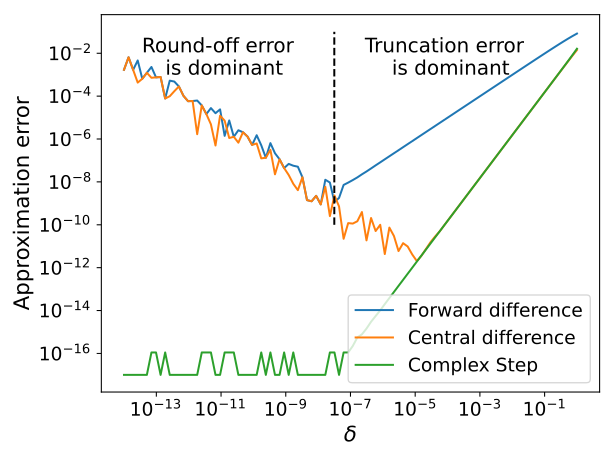
图 7.1:对 f(x):=softplus(x)=log⁡(1+exp⁡(x))f(x)\coloneqq\mathrm{softplus}(x)=\log(1+\exp(x)) 做数值微分,以在 x=1x=1 处近似 f′(x)=logistic(x)f^{\prime}(x)=\mathrm{logistic}(x) 。前向差分法与中心差分法都会同时引入截断误差(当 δ\delta 较大时)和舍入误差(当 δ\delta 较小时)。复步法所受到的舍入误差更小。Figure 7.1: Numerical differentiation of f(x):=softplus(x)=log⁡(1+exp⁡(x))f(x)\coloneqq\mathrm{softplus}(x)=\log(1+\exp(x)), to approximate f′(x)=logistic(x)f^{\prime}(x)=\mathrm{logistic}(x) at x=1x=1. The forward and central difference methods induce both truncation error (for large δ\delta) and round-off error (for small δ\delta). The complex step method enjoys smaller round-off error.

7.2 后向差分7.2 Backward differences

作为另一种选择,我们可以用下式近似方向导数与 JVP:As an alternative, we can approximate the directional derivative and the JVP by

∂f(w)[v]≈f(w)−f(w−δv)δ,\partial f({\bm{w}})[{\bm{v}}]\approx\frac{f({\bm{w}})-f({\bm{w}}-\delta{\bm{v}})}{\delta},

其中 0<δ≪10<\delta\ll 1 为某个取值。该公式称为后向差分。由 2.5.4 节的泰勒展开,我们容易验证 (f(w)−f(w−δv))/δ=∂f(w)[v]+O(δ)(f({\bm{w}})-f({\bm{w}}-\delta{\bm{v}}))/\delta=\partial f({\bm{w}})[{\bm{v}}]+O(\delta) ,因此其截断误差与前向差分相同。for some 0<δ≪10<\delta\ll 1. This formula is called a backward difference. From the Taylor expansion in Section 2.5.4, we easily verify that (f(w)−f(w−δv))/δ=∂f(w)[v]+O(δ)(f({\bm{w}})-f({\bm{w}}-\delta{\bm{v}}))/\delta=\partial f({\bm{w}})[{\bm{v}}]+O(\delta), so that the truncation error is the same as for the forward difference.

7.3 中心差分7.3 Central differences

与前向差分和后向差分这类非对称公式不同,我们可以使用对称公式来近似导数:Rather than using an asymmetric formula to approximate the derivative, as in forward and backward differences, we can use a symmetric formula

∂f(w)[v]≈f(w+δv)−f(w−δv)2δ,\partial f({\bm{w}})[{\bm{v}}]\approx\frac{f({\bm{w}}+\delta{\bm{v}})-f({\bm{w}}-\delta{\bm{v}})}{2\delta},

其中 0<δ≪10<\delta\ll 1 为某个取值。该公式称为中心差分。由 2.5.4 节的泰勒展开,我们有for some 0<δ≪10<\delta\ll 1. This formula is called a central difference. From the Taylor expansion in Section 2.5.4, we have

f(w+δv)−f(w−δv)=\displaystyle f({\bm{w}}+\delta{\bm{v}})-f({\bm{w}}-\delta{\bm{v}})= 2δ∂f(w)[v]+2δ33!∂3f(w)[v,v,v]\displaystyle 2\delta\partial f({\bm{w}})[{\bm{v}}]+\frac{2\delta^{3}}{3!}\partial^{3}f({\bm{w}})[{\bm{v}},{\bm{v}},{\bm{v}}]
+2δ55!∂5f(w)[v,…,v]+…\displaystyle+\frac{2\delta^{5}}{5!}\partial^{5}f({\bm{w}})[{\bm{v}},\dots,{\bm{v}}]+\dots

从而so that

f(w+δv)−f(w−δv)2δ=\displaystyle\frac{f({\bm{w}}+\delta{\bm{v}})-f({\bm{w}}-\delta{\bm{v}})}{2\delta}= ∂f(w)[v]+δ23!∂3f(w)[v,v,v]+…\displaystyle\partial f({\bm{w}})[{\bm{v}}]+\frac{\delta^{2}}{3!}\partial^{3}f({\bm{w}})[{\bm{v}},{\bm{v}},{\bm{v}}]+\ldots
=\displaystyle= ∂f(w)[v]+O(δ2).\displaystyle\partial f({\bm{w}})[{\bm{v}}]+O(\delta^{2}).

可见,偶数阶导数对应的项相互抵消,因而该公式的截断误差达到 O(δ2)O(\delta^{2}) 阶。对任意 δ<1\delta<1,中心差分的截断误差都远小于前向差分或后向差分的截断误差,图 7.1 的经验结果也印证了这一点。We see that the terms corresponding to derivatives of even order canceled out, allowing the formula to achieve O(δ2)O(\delta^{2}) truncation error. For any δ<1\delta<1, the truncation error of the central difference is much smaller than the one of the forward or backward differences as confirmed empirically in Fig. 7.1.

7.4 更高精度的有限差分7.4 Higher-accuracy finite differences

若利用更多的函数取值,还可进一步降低截断误差。前向差分格式可推广为如下形式:The truncation error can be further reduced by making use of additional function evaluations. One can generalize the forward difference scheme by a formula of the form

∂f(w)[v]≈∑t=0patδf(w+tδv)\partial f({\bm{w}})[{\bm{v}}]\approx\sum_{t=0}^{p}\frac{a_{t}}{\delta}f({\bm{w}}+t\delta{\bm{v}})

该式需进行 p+1p+1 次求值。为选取 ata_{t} 并使截断误差达到 O(δp)O(\delta^{p}) 阶,可对求和中的每一项作泰勒展开,得到requiring p+1p+1 evaluations. To select the ata_{t} and reach a truncation error of order O(δp)O(\delta^{p}), we can use a Taylor expansion on each term of the sum to get

∑t=0patδf(w+tδv)\displaystyle\sum_{t=0}^{p}\frac{a_{t}}{\delta}f({\bm{w}}+t\delta{\bm{v}}) =∑t=0pat∑j=0ptjδj−1j!∂jf(w)[v,…,v]+O(δp).\displaystyle=\sum_{t=0}^{p}a_{t}\sum_{j=0}^{p}\frac{t^{j}\delta^{j-1}}{j!}\partial^{j}f({\bm{w}})[{\bm{v}},\ldots,{\bm{v}}]+O(\delta^{p}).

按导数的各阶对求和项分组,便得到 p+1p+1 个系数 a0,…,apa_{0},\ldots,a_{p} 所需满足的 p+1p+1 个方程,即By grouping the terms in the sum for each order of derivative, we obtain a set of p+1p+1 equations to be satisfied by the p+1p+1 coefficients a0,…,apa_{0},\ldots,a_{p}, that is,

a0+a1+…+ap\displaystyle a_{0}+a_{1}+\ldots+a_{p} =0\displaystyle=0
a1+2a2+…+pap\displaystyle a_{1}+2a_{2}+\ldots+pa_{p} =1\displaystyle=1
a1+2ja2+…+pjap\displaystyle a_{1}+2^{j}a_{2}+\ldots+p^{j}a_{p} =0∀j∈{2,…,p}.\displaystyle=0\quad\forall j\in\{2,\ldots,p\}.

该方程组可解析求解,从而定出各系数。后向差分同样可用 ∂f(w)[v]≈∑t=0patδf(w−tδv)\partial f({\bm{w}})[{\bm{v}}]\approx\sum_{t=0}^{p}\frac{a_{t}}{\delta}f({\bm{w}}-t\delta{\bm{v}}) 推广。类似地,中心差分格式可通过This system of equations can be solved analytically to derive the coefficients. Backward differences can be generalized similarly by using ∂f(w)[v]≈∑t=0patδf(w−tδv)\partial f({\bm{w}})[{\bm{v}}]\approx\sum_{t=0}^{p}\frac{a_{t}}{\delta}f({\bm{w}}-t\delta{\bm{v}}). Similarly, the central difference scheme can be generalized by using

∂f(w)[v]≈∑t=−ppatδf(w+tδv),\partial f({\bm{w}})[{\bm{v}}]\approx\sum_{t=-p}^{p}\frac{a_{t}}{\delta}f({\bm{w}}+t\delta{\bm{v}}),

推广,使截断误差达到 O(δ2p)O(\delta^{2p}) 阶。按上述方法解出系数 a−p,…,apa_{-p},\ldots,a_{p},可得 a0=0a_{0}=0。因此,只需进行 2p2p 次求值。to reach a truncation error of order O(δ2p)O(\delta^{2p}). Solving for the coefficients a−p,…,apa_{-p},\ldots,a_{p} as above reveals that a0=0a_{0}=0. Therefore, only 2p2p evaluations are necessary.

7.5 高阶有限差分7.5 Higher-order finite differences

要近似高阶导数,可循类似思路。也就是说,前向差分格式可推广为用下式近似 kk 阶导数:To approximate higher order derivatives, we can follow a similar reasoning. Namely, we can generalize the forward difference scheme to approximate the derivative of order kk by

∂kf(w)[v,…,v]≈∑t=0patδkf(w+tδv).\partial^{k}f({\bm{w}})[{\bm{v}},\ldots,{\bm{v}}]\approx\sum_{t=0}^{p}\frac{a_{t}}{\delta^{k}}f({\bm{w}}+t\delta{\bm{v}}).

与之前一样,可将求和中的各项展开。为使近似只捕捉 kk 阶导数,此时要求系数 ata_{t} 满足As before, we can expand the terms in the sum. For the approximation to capture only the kkth derivative, we now require the coefficients ata_{t} to satisfy

0ja0+1ja1+2ja2+…+pjap\displaystyle 0^{j}a_{0}+1^{j}a_{1}+2^{j}a_{2}+\ldots+p^{j}a_{p} =0∀j∈{0,…,k−1}.\displaystyle=0\quad\forall j\in\{0,\ldots,k-1\}.
0ka0+1ka1+2ka2+…+pkap\displaystyle 0^{k}a_{0}+1^{k}a_{1}+2^{k}a_{2}+\ldots+p^{k}a_{p} =k!\displaystyle=k!
0ja0+1ja1+2ja2+…+pjap\displaystyle 0^{j}a_{0}+1^{j}a_{1}+2^{j}a_{2}+\ldots+p^{j}a_{p} =0∀j∈{k+1,…,p}.\displaystyle=0\quad\forall j\in\{k+1,\ldots,p\}.

由此得到的系数可使截断误差达到 O(δp−k+1)O(\delta^{p-k+1}) 阶,而所需求值次数为 p+1p+1。例如,当 p=k=2p=k=2 时,可将二阶导数近似为With the resulting coefficients, we obtain a truncation error of order O(δp−k+1)O(\delta^{p-k+1}), while making p+1p+1 evaluations. For example, for p=k=2p=k=2, we can approximate the second-order derivative as

∂2f(w)[v,v]≈−(3/2)f(w)+2f(w+δv)−(1/2)f(w+2δv)δ2,\partial^{2}f({\bm{w}})[{\bm{v}},{\bm{v}}]\approx\frac{-(3/2)f({\bm{w}})+2f({\bm{w}}+\delta{\bm{v}})-(1/2)f({\bm{w}}+2\delta{\bm{v}})}{\delta^{2}},

其截断误差为 O(δ)O(\delta) 阶。with a truncation error of order O(δ)O(\delta).

中心差分格式可类似地推广为The central difference scheme can be generalized similarly by

∂kf(w)[v,…,v]≈∑t=−ppatδkf(w+tδv),\partial^{k}f({\bm{w}})[{\bm{v}},\ldots,{\bm{v}}]\approx\sum_{t=-p}^{p}\frac{a_{t}}{\delta^{k}}f({\bm{w}}+t\delta{\bm{v}}),

使截断误差达到 O(δ2p+2−2⌈(k+1)/2⌉)O(\delta^{2p+2-2\lceil(k+1)/2\rceil}) 阶。例如,当 k=2k=2、p=1p=1 时,可得二阶中心差分to reach truncation errors of order O(δ2p+2−2⌈(k+1)/2⌉)O(\delta^{2p+2-2\lceil(k+1)/2\rceil}). For example, for k=2k=2, p=1p=1, we obtain the second-order central difference

∂2f(w)[v,v]≈f(w+δv)+f(w−δv)−2f(w)δ2.\partial^{2}f({\bm{w}})[{\bm{v}},{\bm{v}}]\approx\frac{f({\bm{w}}+\delta{\bm{v}})+f({\bm{w}}-\delta{\bm{v}})-2f({\bm{w}})}{\delta^{2}}.

由泰勒展开可见,这一次奇数阶导数对应的项相互抵消,截断误差为 O(δ2)O(\delta^{2}),而所需求值次数为 33。By using a Taylor expansion we see that, this time, the terms corresponding to derivatives of odd order cancel out and the truncation error is O(δ2)O(\delta^{2}) while requiring 33 evaluations.

7.6 复步法导数7.6 Complex-step derivatives

设 ff 在 CP\mathbb{C}^{P} 上良定义,后者即 PP 维复数的空间。记虚数单位为 i=−1i=\sqrt{-1}。于是,ff 的泰勒展开为Suppose ff is well defined on CP\mathbb{C}^{P}, the space of PP-dimensional complex numbers. Let us denote the imaginary unit by i=−1i=\sqrt{-1}. Then, the Taylor expansion of ff reads

f(w+(iδ)v)=\displaystyle f({\bm{w}}+(i\delta){\bm{v}})= f(w)+(iδ)∂f(w)[v]+(iδ)22∂2f(w)[v,v]\displaystyle f({\bm{w}})+(i\delta)\partial f({\bm{w}})[{\bm{v}}]+\frac{(i\delta)^{2}}{2}\partial^{2}f({\bm{w}})[{\bm{v}},{\bm{v}}]
+(iδ)33!∂3f(w)[v,v,v]+…\displaystyle+\frac{(i\delta)^{3}}{3!}\partial^{3}f({\bm{w}})[{\bm{v}},{\bm{v}},{\bm{v}}]+\dots
=\displaystyle= f(w)+(iδ)∂f(w)[v]−δ22∂2f(w)[v,v]\displaystyle f({\bm{w}})+(i\delta)\partial f({\bm{w}})[{\bm{v}}]-\frac{\delta^{2}}{2}\partial^{2}f({\bm{w}})[{\bm{v}},{\bm{v}}]
−iδ33!∂3f(w)[v,v,v]+….\displaystyle-\frac{i\delta^{3}}{3!}\partial^{3}f({\bm{w}})[{\bm{v}},{\bm{v}},{\bm{v}}]+\dots\quad.

可见,实部对应偶数阶项,虚部对应奇数阶项。由此可得We see that the real part corresponds to even-degree terms and the imaginary part corresponds to odd-degree terms. We therefore obtain

Re⁡(f(w+(iδ)v))=f(w)+O(δ2)\operatorname{Re}(f({\bm{w}}+(i\delta){\bm{v}}))=f({\bm{w}})+O(\delta^{2})

以及and

Im⁡(f(w+(iδ)v)δ)=∂f(w)[v]+O(δ2).\operatorname{Im}\left(\frac{f({\bm{w}}+(i\delta){\bm{v}})}{\delta}\right)=\partial f({\bm{w}})[{\bm{v}}]+O(\delta^{2}).

这表明,我们可以用如下近似来计算方向导数:This suggests that we can compute directional derivatives using the approximation

∂f(w)[v]≈Im⁡(f(w+(iδ)v)δ),\partial f({\bm{w}})[{\bm{v}}]\approx\operatorname{Im}\left(\frac{f({\bm{w}}+(i\delta){\bm{v}})}{\delta}\right),

其中 0<δ≪10<\delta\ll 1。这一方法称为复步法导数近似 [186, 130]。for 0<δ≪10<\delta\ll 1. This is called the complex-step derivative approximation [186, 130].

与前向差分、后向差分和中心差分不同,这里只需调用一次函数。对复数调用一次函数的开销,大约是对实数调用一次函数的两倍。不过,由于不再需要计算函数之差,复步法导数近似通常具有更小的舍入误差,如图 7.1 所示。话虽如此,该方法的一个缺点是:实现函数 ff 的程序中,所有基本操作都必须在复数上良定义,例如借助运算符重载来实现。Contrary to forward, backward and central differences, we see that only a single function call is necessary. A function call on complex numbers may take roughly twice the cost of a function call on real numbers. However, thanks to the fact that a difference of functions is no longer needed, the complex-step derivative approximation usually enjoys smaller round-off error as illustrated in Fig. 7.1. That said, one drawback of the method is that all elementary operations within the program implementing the function ff must be well-defined on complex numbers, e.g., using overloading.

7.7 复杂度7.7 Complexity

下面从函数求值次数的角度,讨论有限差分与复步法导数的计算复杂度。具体而言,由于这是机器学习中最常见的情形,我们考虑单个 M=1M=1 输出的情况,即要对一个函数 f ⁣:RP→Rf\colon\mathbb{R}^{P}\to\mathbb{R} 求导。无论采用前向差分、后向差分还是中心差分,计算任意方向 v{\bm{v}} 上的方向导数 ∂f(w)[v]\partial f({\bm{w}})[{\bm{v}}] 的计算复杂度都相当于调用 ff 两次。至于梯度 ∇f(w)\nabla f({\bm{w}}) 的计算,我们可以利用(见定义 2.2.4)We now discuss the computational complexity in terms of function evaluations of finite differences and complex-step derivatives. For concreteness, as this is the most common use case in machine learning, we discuss the case of a single M=1M=1 output, i.e., we want to differentiate a function f ⁣:RP→Rf\colon\mathbb{R}^{P}\to\mathbb{R}. Whether we use forward, backward or central differences, the computational complexity of computing the directional derivative ∂f(w)[v]\partial f({\bm{w}})[{\bm{v}}] in any direction v{\bm{v}} amounts to two calls to ff. For computing the gradient ∇f(w)\nabla f({\bm{w}}), we can use (see Definition 2.2.4) that

[∇f(w)]j=⟨∇f(w),ej⟩=∂f(w)[ej],[\nabla f({\bm{w}})]_{j}=\langle\nabla f({\bm{w}}),{\bm{e}}_{j}\rangle=\partial f({\bm{w}})[{\bm{e}}_{j}],

对于 j∈[P]j\in[P]。因此,若采用前向差分或后向差分,计算梯度需要 P+1P+1 次函数调用;若采用中心差分,则需要 2P2P 次函数调用。对于复步法近似,则需要 PP 次复函数调用。这些复杂度总结于表 7.1。for j∈[P]j\in[P]. For forward and backward differences, we therefore need P+1P+1 function calls to compute the gradient, while we need 2P2P function calls for central differences. For the complex step approximation, we need PP complex function calls. We summarize the complexities in Table 7.1.

表 7.1:以函数求值次数表示的有限差分与复步法导数在计算函数 f ⁣:RP→Rf\colon\mathbb{R}^{P}\to\mathbb{R} 的方向导数和梯度时的计算复杂度。Table 7.1: Computational complexity in number of function evaluations for computing the directional derivative and the gradient of a function f ⁣:RP→Rf\colon\mathbb{R}^{P}\to\mathbb{R} by finite differences and complex step derivatives.
方向导数Directional derivative 梯度Gradient
前向差分Forward difference 22 P+1P+1
后向差分Backward difference 22 P+1P+1
中心差分Central difference 22 2P2P
复步法Complex step 11 PP

7.8 小结7.8 Summary

  • •

    有限差分是一种仅凭函数求值即可数值计算导数的简便方法。Finite differences are a simple way to numerically compute derivatives using only function evaluations.

  • •

    中心差分的截断误差小于前向差分和后向差分。若愿意付出更多函数求值的代价,还可进一步减小截断误差。Central differences achieve smaller truncation error than forward and backward differences. It is possible to achieve smaller truncation error, at the cost of more function evaluations.

  • •

    复步法导数的舍入误差小于中心差分,但要求函数本身以及实现该函数的程序在复数上良定义。Complex-step derivatives achieve smaller round-off error than central differences but require the function and the program implementing it to be well-defined on complex numbers.

  • •

    然而,无论采用哪种方法,有限差分所需的函数调用次数都与维数成正比。因此,在维度动辄数百万乃至数十亿的机器学习中,这类方法鲜有使用。有限差分的主要应用场景因而有两类:i)低维黑箱函数;ii)测试用途(例如检查梯度函数是否实现正确)。However, whatever the method used, finite differences require a number of function calls that is proportional to the number of dimensions. They are therefore seldom used in machine learning, where there can be millions or billions of dimensions. The main use cases of finite differences are therefore i) for blackbox functions of low dimension and ii) for test purposes (e.g., checking that a gradient function is correctly implemented).

  • •

    在现代机器学习中,主要依靠的是自动微分,因为它能够利用函数的复合结构。这正是下一章要研究的内容。For modern machine learning, the main workhorse is automatic differentiation, as it leverages the compositional structure of functions. This is what we study in the next chapter.