目录概率学习

第 3 章 概率学习Chapter 3 Probabilistic learning

本章回顾如何进行概率学习,并介绍指数族分布,因为它们在本书中起着关键作用。In this chapter, we review how to perform probabilistic learning. We also introduce exponential family distributions, as they play a key role in this book.

3.1 概率分布3.1 Probability distributions

3.1.1 离散概率分布Discrete probability distributions

集合 Y\mathcal{Y} 上的离散概率分布由其概率质量函数(PMF)p ⁣:Y→[0,1]p\colon\mathcal{Y}\to[0,1] 给定。于是,y∈Y{\bm{y}}\in\mathcal{Y} 的概率定义为A discrete probability distribution over a set Y\mathcal{Y} is specified by its probability mass function (PMF) p ⁣:Y→[0,1]p\colon\mathcal{Y}\to[0,1]. The probability of y∈Y{\bm{y}}\in\mathcal{Y} is then defined by

P(Y=y):=p(y),\mathbb{P}(Y={\bm{y}})\coloneqq p({\bm{y}}),

其中 YY 表示随机变量。当 YY 服从分布 pp 时,我们记作 Y∼pY\sim p(这里略微滥用记号:用同一个字母 pp 同时表示分布与 PMF)。于是,ϕ(Y)\phi(Y) 的期望为(其中 Y∼pY\sim p,ϕ ⁣:Y→RM\phi\colon\mathcal{Y}\to\mathbb{R}^{M})where YY denotes a random variable. When YY follows a distribution pp, we write Y∼pY\sim p (with some abuse of notation, we use the same letter pp to denote the distribution and the PMF). The expectation of ϕ(Y)\phi(Y), where Y∼pY\sim p and ϕ ⁣:Y→RM\phi\colon\mathcal{Y}\to\mathbb{R}^{M}, is then

E[ϕ(Y)]=∑y∈Yp(y)ϕ(y),\mathbb{E}[\phi(Y)]=\sum_{{\bm{y}}\in\mathcal{Y}}p({\bm{y}})\phi({\bm{y}}),

其方差(一维变量情形)为its variance (for one-dimensional variables) is

V[ϕ(Y)]=E[(ϕ(Y)−E[ϕ(Y)])2]=∑y∈Yp(y)(ϕ(y)−E[ϕ(Y)])2\mathbb{V}[\phi(Y)]=\mathbb{E}[(\phi(Y)-\mathbb{E}[\phi(Y)])^{2}]=\sum_{{\bm{y}}\in\mathcal{Y}}p({\bm{y}})(\phi({\bm{y}})-\mathbb{E}[\phi(Y)])^{2}

而其众数为and its mode is

arg max⁡y∈Yp(y).\argmax_{{\bm{y}}\in\mathcal{Y}}p({\bm{y}}).

集合 Y\mathcal{Y} 上两个离散分布之间的 Kullback-Leibler(KL)散度(亦称相对熵),在相应 PMF 分别为 pp 与 qq 时,是如下定义的统计“距离”The Kullback-Leibler (KL) divergence (also known as relative entropy) between two discrete distributions over Y\mathcal{Y}, with associated PMFs pp and qq, is the statistical “distance” defined by

KL(p,q):=∑y∈Yp(y)log⁡(p(y)q(y))=EY∼plog⁡(p(Y)q(Y)).\mathrm{KL}(p,q)\coloneqq\sum_{{\bm{y}}\in\mathcal{Y}}p({\bm{y}})\log\left(\frac{p({\bm{y}})}{q({\bm{y}})}\right)=\mathbb{E}_{Y\sim p}\log\left(\frac{p(Y)}{q(Y)}\right).

3.1.2 连续概率分布Continuous probability distributions

集合 Y\mathcal{Y} 上的连续概率分布由其概率密度函数(PDF)p ⁣:Y→R+p\colon\mathcal{Y}\to\mathbb{R}_{+} 给定。于是,A⊆Y\mathcal{A}\subseteq\mathcal{Y} 的概率为A continuous probability distribution over Y\mathcal{Y} is specified by its probability density function (PDF) p ⁣:Y→R+p\colon\mathcal{Y}\to\mathbb{R}_{+}. The probability of A⊆Y\mathcal{A}\subseteq\mathcal{Y} is then

P(Y∈A)=∫Ap(y)dy.\mathbb{P}(Y\in\mathcal{A})=\int_{\mathcal{A}}p(y)dy.

期望、方差与 KL 散度的定义均与离散情形类似,只需把 ∑y∈Y\sum_{{\bm{y}}\in\mathcal{Y}} 换作 ∫Y\int_{\mathcal{Y}}。具体而言,ϕ(Y)\phi(Y) 的期望为The expectation, variance and KL divergence are defined analogously to the discrete setting, simply replacing ∑y∈Y\sum_{{\bm{y}}\in\mathcal{Y}} with ∫Y\int_{\mathcal{Y}}. Specifically, the expectation of ϕ(Y)\phi(Y) is

E[ϕ(Y)]=∫Yp(y)ϕ(y)dy,\mathbb{E}[\phi(Y)]=\int_{\mathcal{Y}}p(y)\phi(y)dy,

方差为the variance is

V[ϕ(Y)]=E[(ϕ(Y)−E[ϕ(Y)])2]=∫Yp(y)(ϕ(y)−E[ϕ(Y)])2dy\mathbb{V}[\phi(Y)]=\mathbb{E}[(\phi(Y)-\mathbb{E}[\phi(Y)])^{2}]=\int_{\mathcal{Y}}p(y)(\phi(y)-\mathbb{E}[\phi(Y)])^{2}dy

而 KL 散度为and the KL divergence is

KL(p,q):=∫Yp(y)log⁡(p(y)q(y))dy=EY∼plog⁡(p(Y)q(Y)).\mathrm{KL}(p,q)\coloneqq\int_{\mathcal{Y}}p(y)\log\left(\frac{p(y)}{q(y)}\right)dy=\mathbb{E}_{Y\sim p}\log\left(\frac{p(Y)}{q(Y)}\right).

众数则定义为 PDF 的 argmax。The mode is defined as the argmax of the PDF.

当 Y=R\mathcal{Y}=\mathbb{R} 时,还可定义累积分布函数(CDF)When Y=R\mathcal{Y}=\mathbb{R}, we can also define the cumulative distribution function (CDF)

P(Y≤b)=∫−∞bp(y)dy.\mathbb{P}(Y\leq b)=\int_{-\infty}^{b}p(y)dy.

于是,YY 落入半闭区间 (a,b](a,b] 内的概率为The probability of YY lying in the semi-closed interval (a,b](a,b] is then

P(a<Y≤b)=P(Y≤b)−P(Y≤a).\mathbb{P}(a<Y\leq b)=\mathbb{P}(Y\leq b)-\mathbb{P}(Y\leq a).

3.2 最大似然估计3.2 Maximum likelihood estimation

3.2.1 负对数似然Negative log-likelihood

我们已经看到,集合 Y\mathcal{Y} 上的概率分布由 p(y)p({\bm{y}}) 给定:对离散变量它称为概率质量函数(PMF),对连续变量则称为概率密度函数(PDF)。实际中,生成数据的真实分布 pp 未知,我们希望用一个带参数 λ∈Λ{\bm{\lambda}}\in\Lambda 的分布 pλp_{\bm{\lambda}} 来近似它。现给定一组有限的独立同分布观测 y1,…,yN{\bm{y}}_{1},\dots,{\bm{y}}_{N},应如何将 λ∈Λ{\bm{\lambda}}\in\Lambda 拟合到数据?这可以通过最大化数据的似然来实现,即我们求解We saw that a probability distribution over Y\mathcal{Y} is specified by p(y)p({\bm{y}}), which is called the probability mass function (PMF) for discrete variables or the probability density function (PDF) for continuous variables. In practice, the true distribution pp generating the data is unknown and we wish to approximate it with a distribution pλp_{\bm{\lambda}}, with parameters λ∈Λ{\bm{\lambda}}\in\Lambda. Given a finite set of i.i.d. observations y1,…,yN{\bm{y}}_{1},\dots,{\bm{y}}_{N}, how do we fit λ∈Λ{\bm{\lambda}}\in\Lambda to the data? This can be done by maximizing the likelihood of the data, i.e., we seek to solve

λ^N:=arg max⁡λ∈Λ∏i=1Npλ(yi).\widehat{\bm{\lambda}}_{N}\coloneqq\argmax_{{\bm{\lambda}}\in\Lambda}\prod_{i=1}^{N}p_{{\bm{\lambda}}}({\bm{y}}_{i}).

这称为最大似然估计(MLE)。由于 log⁡\log 函数单调递增,此举等价于最小化负对数似然,即我们有This is known as maximum likelihood estimation (MLE). Because the log⁡\log function is monotonically increasing, this is equivalent to minimizing the negative log-likelihood, i.e., we have

λ^N=arg min⁡λ∈Λ−∑i=1Nlog⁡pλ(yi).\widehat{\bm{\lambda}}_{N}=\argmin_{{\bm{\lambda}}\in\Lambda}-\sum_{i=1}^{N}\log p_{{\bm{\lambda}}}({\bm{y}}_{i}).
例 3.2.1(正态分布的最大似然估计)。Example 3.2.1 (MLE for the normal distribution).
设 pλp_{\bm{\lambda}} 为正态分布,其参数为 λ=(μ,σ){\bm{\lambda}}=(\mu,\sigma),即Suppose we set pλp_{\bm{\lambda}} to the normal distribution with parameters λ=(μ,σ){\bm{\lambda}}=(\mu,\sigma), i.e., pλ(y):=1σ2πexp⁡(−12(y−μσ)2).p_{\bm{\lambda}}(y)\coloneqq\frac{1}{\sigma\sqrt{2\pi}}\exp\left(-\frac{1}{2}\left(\frac{y-\mu}{\sigma}\right)^{2}\right). 于是,给定观测 y1,…,yNy_{1},\dots,y_{N},μ\mu 与 σ2\sigma^{2} 的最大似然估计(MLE)分别为样本均值与样本方差。Then, given observations y1,…,yNy_{1},\dots,y_{N}, the MLEs for μ\mu and σ2\sigma^{2} are the sample mean and the sample variance, respectively.

3.2.2 关于 Kullback-Leibler 散度的一致性Consistency w.r.t. the Kullback-Leibler divergence

众所周知,MLE 在 Kullback-Leibler 散度意义下是一致的。也就是说,记真实分布为 pp,并且It is well-known that the MLE is consistent, in the sense of the Kullback-Leibler divergence. That is, denoting the true distribution pp and

λ∞:=arg min⁡λ∈ΛKL(p,pλ){\bm{\lambda}}_{\infty}\coloneqq\argmin_{{\bm{\lambda}}\in\Lambda}\mathrm{KL}(p,p_{\bm{\lambda}})

其中,where

KL(p,pλ)=EY∼plog⁡(p(Y)pλ(Y)),\mathrm{KL}(p,p_{\bm{\lambda}})=\mathbb{E}_{Y\sim p}\log\left(\frac{p(Y)}{p_{\bm{\lambda}}(Y)}\right),

那么,对观测取期望后有 λ^N→λ∞\widehat{\bm{\lambda}}_{N}\to{\bm{\lambda}}_{\infty},当 N→∞N\to\infty 时成立。这一结论可通过使用then λ^N→λ∞\widehat{\bm{\lambda}}_{N}\to{\bm{\lambda}}_{\infty} in expectation over the observations, as N→∞N\to\infty. This can be seen by using

KL(p,pλ)≈1N∑i=1Nlog⁡(p(yi)pλ(yi))=1N∑i=1N(log⁡p(yi)−log⁡pλ(yi))\mathrm{KL}(p,p_{\bm{\lambda}})\approx\frac{1}{N}\sum_{i=1}^{N}\log\left(\frac{p({\bm{y}}_{i})}{p_{\bm{\lambda}}({\bm{y}}_{i})}\right)=\frac{1}{N}\sum_{i=1}^{N}\left(\log p({\bm{y}}_{i})-\log p_{\bm{\lambda}}({\bm{y}}_{i})\right)

以及大数定律得到。and the law of large numbers.

3.3 概率监督学习3.3 Probabilistic supervised learning

3.3.1 条件概率分布Conditional probability distributions

在机器学习中,很多时候我们希望针对某个输入 x∈X{\bm{x}}\in\mathcal{X} 定义条件概率 P(Y=y∣X=x)\mathbb{P}(Y={\bm{y}}|X={\bm{x}}),而不是针对某个 y∈Y{\bm{y}}\in\mathcal{Y} 定义概率 P(Y=y)\mathbb{P}(Y={\bm{y}})。这可以通过归约为无条件概率分布来实现,Many times in machine learning, instead of a probability P(Y=y)\mathbb{P}(Y={\bm{y}}) for some y∈Y{\bm{y}}\in\mathcal{Y}, we wish to define a conditional probability P(Y=y∣X=x)\mathbb{P}(Y={\bm{y}}|X={\bm{x}}), for some input x∈X{\bm{x}}\in\mathcal{X}. This can be achieved by reduction to an unconditional probability distribution,

P(Y=y∣X=x):=pλ(y)\mathbb{P}(Y={\bm{y}}|X={\bm{x}})\coloneqq p_{\bm{\lambda}}({\bm{y}})

其中where

λ:=f(x,w){\bm{\lambda}}\coloneqq f({\bm{x}},{\bm{w}})

而 ff 是一个带有模型参数 w∈W{\bm{w}}\in\mathcal{W} 的模型函数。也就是说,ff 并非从 X\mathcal{X} 到 Y\mathcal{Y} 的确定性函数,而是从 X\mathcal{X} 到 Λ\Lambda 的函数,其中后者是与输入相关联的输出分布所允许的分布参数集合。and ff is a model function with model parameters w∈W{\bm{w}}\in\mathcal{W}. That is, rather than being a deterministic function from X\mathcal{X} to Y\mathcal{Y}, ff is a function from X\mathcal{X} to Λ\Lambda, the set of permissible distribution parameters of the output distribution associated with the input.

我们要强调,λ{\bm{\lambda}} 可以是单个参数,也可以是一组参数的集合。例如,在 伯努利分布中,λ=π\lambda=\pi;而在一元正态分布中,λ=(μ,σ){\bm{\lambda}}=(\mu,\sigma)。We emphasize that λ{\bm{\lambda}} could be a single parameter or a collection of parameters. For instance, in the Bernoulli distribution, λ=π\lambda=\pi, while in the univariate normal distribution, λ=(μ,σ){\bm{\lambda}}=(\mu,\sigma).

在 3.4 节以及本书其余部分,当 θ{\bm{\theta}} 是指数族分布的典范参数时,我们也会使用记号 pθp_{\bm{\theta}} 来代替 pλp_{\bm{\lambda}}。In Section 3.4 and throughout this book, we will also use the notation pθp_{\bm{\theta}} instead of pλp_{\bm{\lambda}} when θ{\bm{\theta}} are the canonical parameters of an exponential family distribution.

3.3.2 推断Inference

这种概率方法的主要优势在于,我们的预测模型比仅仅学习一个从 X\mathcal{X} 到 Y\mathcal{Y} 的函数要丰富得多。现在我们可以获得 Y\mathcal{Y} 中所有可能结果的整个分布,并计算各种统计量:The main advantage of this probabilistic approach is that our prediction model is much richer than if we just learned a function from X\mathcal{X} to Y\mathcal{Y}. We now have access to the whole distribution over possible outcomes in Y\mathcal{Y} and can compute various statistics:

  • •

    概率:P(Y=y∣X=x)\mathbb{P}(Y={\bm{y}}|X={\bm{x}}) 或 P(Y∈A∣X=x)\mathbb{P}(Y\in\mathcal{A}|X={\bm{x}}),Probability: P(Y=y∣X=x)\mathbb{P}(Y={\bm{y}}|X={\bm{x}}) or P(Y∈A∣X=x)\mathbb{P}(Y\in\mathcal{A}|X={\bm{x}}),

  • •

    期望:对于某个函数 ϕ\phi,E[ϕ(Y)∣X=x]\mathbb{E}[\phi(Y)|X={\bm{x}}],Expectation: E[ϕ(Y)∣X=x]\mathbb{E}[\phi(Y)|X={\bm{x}}] for some function ϕ\phi,

  • •

    方差:V[ϕ(Y)∣X=x]\mathbb{V}[\phi(Y)|X={\bm{x}}],Variance: V[ϕ(Y)∣X=x]\mathbb{V}[\phi(Y)|X={\bm{x}}],

  • •

    众数:arg max⁡y∈Ypλ(y)\argmax_{{\bm{y}}\in\mathcal{Y}}p_{\bm{\lambda}}({\bm{y}})。Mode: arg max⁡y∈Ypλ(y)\argmax_{{\bm{y}}\in\mathcal{Y}}p_{\bm{\lambda}}({\bm{y}}).

现在我们回顾一些概率分布,它们适用于二分类、多分类、回归、多元回归和整数回归。在下文中,为使记号更简洁,我们省略对 x{\bm{x}} 的依赖。We now review probability distributions useful for binary classification, multiclass classification, regression, multivariate regression, and integer regression. In the following, to make the notation more lightweight, we omit the dependence on x{\bm{x}}.

3.3.3 二分类Binary classification

对于二值结果,其中 Y={0,1}\mathcal{Y}=\{0,1\},我们可以使用一个伯努利分布,其参数为For binary outcomes, where Y={0,1}\mathcal{Y}=\{0,1\}, we can use a Bernoulli distribution with parameter

λ:=π∈[0,1].\lambda\coloneqq\pi\in[0,1].

当随机变量 YY 服从参数为 π\pi 的伯努利分布时,我们记作When a random variable YY is distributed according to a Bernoulli distribution with parameter π\pi, we write

Y∼Bernoulli(π).Y\sim\mathrm{Bernoulli}(\pi).

该分布的概率质量函数为The PMF of this distribution is

pπ(y):={πif y=11−πif y=0.p_{\pi}(y)\coloneqq\begin{cases}\pi&\text{if }y=1\\ 1-\pi&\text{if }y=0\end{cases}.

伯努利分布是单次试验的二项分布。由于 y∈{0,1}y\in\{0,1\},概率质量函数可改写为The Bernoulli distribution is a binomial distribution with a single trial. Since y∈{0,1}y\in\{0,1\}, the PMF can be rewritten as

pπ(y)=πy(1−π)1−y.p_{\pi}(y)=\pi^{y}(1-\pi)^{1-y}.

其均值为The mean is

E[Y]=π=P(Y=1)\mathbb{E}[Y]=\pi=\mathbb{P}(Y=1)

其方差为and the variance is

V[Y]=π(1−π)=P(Y=1)P(Y=0).\mathbb{V}[Y]=\pi(1-\pi)=\mathbb{P}(Y=1)\mathbb{P}(Y=0).
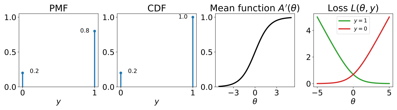
图 3.1:伯努利分布,其概率质量函数与累积分布函数在此以参数 π=0.8\pi=0.8 展示。其均值函数为 π=A′(θ)=logistic(θ)=11+exp⁡(−θ)\pi=A^{\prime}(\theta)=\mathrm{logistic}(\theta)=\frac{1}{1+\exp(-\theta)},其中 θ\theta 例如是神经网络的输出。负对数似然导出 logistic 损失,L(θ,y)=softplus(θ)−θy=log⁡(1+exp⁡(θ))−θyL(\theta,y)=\mathrm{softplus}(\theta)-\theta y=\log(1+\exp(\theta))-\theta y。损失曲线在 y∈{0,1}y\in\{0,1\} 下展示。Figure 3.1: The Bernoulli distribution, whose PMF and CDF are here illustrated with parameter π=0.8\pi=0.8. Its mean function is π=A′(θ)=logistic(θ)=11+exp⁡(−θ)\pi=A^{\prime}(\theta)=\mathrm{logistic}(\theta)=\frac{1}{1+\exp(-\theta)}, where θ\theta is for instance the output of a neural network. The negative log-likelihood leads to the logistic loss, L(θ,y)=softplus(θ)−θy=log⁡(1+exp⁡(θ))−θyL(\theta,y)=\mathrm{softplus}(\theta)-\theta y=\log(1+\exp(\theta))-\theta y. The loss curve is shown for y∈{0,1}y\in\{0,1\}.

使用 sigmoid 进行参数化Parameterization using a sigmoid

由于 伯努利分布的参数 π\pi 需属于 [0,1][0,1],我们通常使用 sigmoid 函数(4.4.3 节),例如以 logistic 函数作为输出层:Since the parameter π\pi of a Bernoulli distribution needs to belong to [0,1][0,1], we typically use a sigmoid function (Section 4.4.3), such as a logistic function as the output layer:

π:=f(x,w):=logistic(g(x,w)),\pi\coloneqq f({\bm{x}},{\bm{w}})\coloneqq\mathrm{logistic}(g({\bm{x}},{\bm{w}})),

其中 g ⁣:X×W→Rg\colon\mathcal{X}\times\mathcal{W}\to\mathbb{R} 例如是神经网络,且where g ⁣:X×W→Rg\colon\mathcal{X}\times\mathcal{W}\to\mathbb{R} is for example a neural network and

logistic(a):=11+exp⁡(−a)∈(0,1).\mathrm{logistic}(a)\coloneqq\frac{1}{1+\exp(-a)}\in(0,1).

当 gg 关于 w{\bm{w}} 为线性时,这称为二分类 logistic 回归。When gg is linear in w{\bm{w}}, this is known as binary logistic regression.

注 3.3.1(与 logistic 分布的联系)。Remark 3.3.1 (Link with the logistic distribution).
均值和尺度参数分别为 μ\mu 与 σ\sigma 的 logistic 分布是一个连续概率分布,其 PDF 为The logistic distribution with mean and scale parameters μ\mu and σ\sigma is a continuous probability distribution with PDF pμ,σ(u):=1σp0,1(u−μσ)p_{\mu,\sigma}(u)\coloneqq\frac{1}{\sigma}p_{0,1}\left(\frac{u-\mu}{\sigma}\right) 其中where p0,1(z):=exp⁡(−z)(1+exp⁡(−z))2.p_{0,1}(z)\coloneqq\frac{\exp(-z)}{(1+\exp(-z))^{2}}. 若随机变量 UU 服从参数为 μ\mu 与 σ\sigma 的 logistic 分布,则记作 U∼Logistic(μ,σ)U\sim\mathrm{Logistic}(\mu,\sigma)。U∼Logistic(μ,σ)U\sim\mathrm{Logistic}(\mu,\sigma) 的 CDF 为If a random variable UU follows a logistic distribution with parameters μ\mu and σ\sigma, we write U∼Logistic(μ,σ)U\sim\mathrm{Logistic}(\mu,\sigma). The CDF of U∼Logistic(μ,σ)U\sim\mathrm{Logistic}(\mu,\sigma) is P(U≤u)=∫−∞upμ,σ(t)dt=logistic(u−μσ).\mathbb{P}(U\leq u)=\int_{-\infty}^{u}p_{\mu,\sigma}(t)dt=\mathrm{logistic}\left(\frac{u-\mu}{\sigma}\right). 因此,若Therefore, if U∼Logistic(μ,σ)U\sim\mathrm{Logistic}(\mu,\sigma) 且and Y∼Bernoulli(logistic(u−μσ)),Y\sim\mathrm{Bernoulli}\left(\mathrm{logistic}\left(\frac{u-\mu}{\sigma}\right)\right), 则then P(Y=1)=P(U≤u).\mathbb{P}(Y=1)=\mathbb{P}(U\leq u). 这里,UU 可解释为一个潜在的连续变量,而 uu 则可解释为一个阈值。Here, UU can be interpreted as a latent continuous variable and uu as a threshold.

3.3.4 多分类Multiclass classification

对于有 MM 种可能取值的分类结果,其中 Y=[M]\mathcal{Y}=[M],我们可以使用一个分类分布,其参数为For categorical outcomes with MM possible choices, where Y=[M]\mathcal{Y}=[M], we can use a categorical distribution with parameters

λ:=π∈△M,{\bm{\lambda}}\coloneqq{\bm{\pi}}\in\triangle^{M},

的 分类分布,其中我们定义概率单纯形where we define the probability simplex

△M:={π∈R+M ⁣:⟨π,1⁡⟩=1},\triangle^{M}\coloneqq\{{\bm{\pi}}\in\mathbb{R}_{+}^{M}\colon\langle{\bm{\pi}},\operatorname{\mathbf{1}}\rangle=1\},

即有效离散概率分布的集合。当 YY 服从参数为 π{\bm{\pi}} 的分类分布时,我们记作i.e., the set of valid discrete probability distributions. When YY follows a categorical distribution with parameter π{\bm{\pi}}, we write

Y∼Categorical(π).Y\sim\mathrm{Categorical}({\bm{\pi}}).

分类分布的概率质量函数为The PMF of the categorical distribution is

pπ(y):=⟨π,ϕ(y)⟩=πy,p_{\bm{\pi}}(y)\coloneqq\langle{\bm{\pi}},\phi(y)\rangle=\pi_{y},

其中where

ϕ(y):=ey\phi(y)\coloneqq{\bm{e}}_{y}

是坐标 y∈[M]y\in[M] 的标准基向量。is the standard basis vector for the coordinate y∈[M]y\in[M].

由于 YY 是 分类变量,计算 YY 的期望并无意义,但我们可以计算 ϕ(Y)=eY\phi(Y)={\bm{e}}_{Y} 的期望,Since YY is a categorical variable, it does not make sense to compute the expectation of YY but we can compute that of ϕ(Y)=eY\phi(Y)={\bm{e}}_{Y},

EY∼pπ[ϕ(Y)]=π.\mathbb{E}_{Y\sim p_{\bm{\pi}}}[\phi(Y)]={\bm{\pi}}.

因此,与 伯努利分布的情形相同,此处均值与概率分布(由向量 π{\bm{\pi}} 表示)也是一致的。Therefore, as was also the case for the Bernoulli distribution, the mean and the probability distribution (represented by the vector π{\bm{\pi}}) are the same in this case.

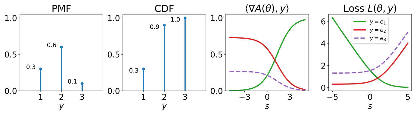
图 3.2:分类分布,其概率质量函数与累积分布函数在此以参数 π=(0.3,0.6,0.1){\bm{\pi}}=(0.3,0.6,0.1) 展示。其均值函数为 π=∇A(θ)=softargmax(θ){\bm{\pi}}=\nabla A({\bm{\theta}})=\mathrm{softargmax}({\bm{\theta}}),其中 θ∈RM{\bm{\theta}}\in\mathbb{R}^{M} 例如是神经网络的输出。为便于说明,此处我们固定 θ=(s,1,0){\bm{\theta}}=(s,1,0),仅改变 ss。由于均值函数 ∇A(θ)\nabla A({\bm{\theta}}) 属于 R3\mathbb{R}^{3},我们选择对 i∈{1,2,3}i\in\{1,2,3\} 展示 ⟨∇A(θ),ei⟩=∇A(θ)i\langle\nabla A({\bm{\theta}}),{\bm{e}}_{i}\rangle=\nabla A({\bm{\theta}})_{i}。负对数似然导出 logistic 损失,L(θ,y)=logsumexp(θ)−⟨θ,y⟩L({\bm{\theta}},{\bm{y}})=\mathrm{logsumexp}({\bm{\theta}})-\langle{\bm{\theta}},{\bm{y}}\rangle。损失曲线在 y∈{e1,e2,e3}{\bm{y}}\in\{{\bm{e}}_{1},{\bm{e}}_{2},{\bm{e}}_{3}\} 下展示,同样固定 θ=(s,1,0){\bm{\theta}}=(s,1,0) 并改变 ss。Figure 3.2: The categorical distribution, whose PMF and CDF are here illustrated with parameter π=(0.3,0.6,0.1){\bm{\pi}}=(0.3,0.6,0.1). Its mean function is π=∇A(θ)=softargmax(θ){\bm{\pi}}=\nabla A({\bm{\theta}})=\mathrm{softargmax}({\bm{\theta}}), where θ∈RM{\bm{\theta}}\in\mathbb{R}^{M} is for instance the output of a neural network. Here, for illustration purpose, we choose to set θ=(s,1,0){\bm{\theta}}=(s,1,0) and vary only ss. Since the mean function ∇A(θ)\nabla A({\bm{\theta}}) belongs to R3\mathbb{R}^{3}, we choose to display ⟨∇A(θ),ei⟩=∇A(θ)i\langle\nabla A({\bm{\theta}}),{\bm{e}}_{i}\rangle=\nabla A({\bm{\theta}})_{i}, for i∈{1,2,3}i\in\{1,2,3\}. The negative log-likelihood leads to the logistic loss, L(θ,y)=logsumexp(θ)−⟨θ,y⟩L({\bm{\theta}},{\bm{y}})=\mathrm{logsumexp}({\bm{\theta}})-\langle{\bm{\theta}},{\bm{y}}\rangle. The loss curve is shown for y∈{e1,e2,e3}{\bm{y}}\in\{{\bm{e}}_{1},{\bm{e}}_{2},{\bm{e}}_{3}\}, again with θ=(s,1,0){\bm{\theta}}=(s,1,0) and varying ss.

使用 softargmax 进行参数化Parameterization using a softargmax

分类分布 π{\bm{\pi}} 的参数向量必须属于 △M\triangle^{M},因此我们通常以 softargmax 作为输出层:Since the parameter vector π{\bm{\pi}} of a categorical distribution needs to belong to △M\triangle^{M}, we typically use a softargmax as the output layer:

π:=f(x,w):=softargmax(g(x,w)),{\bm{\pi}}\coloneqq f({\bm{x}},{\bm{w}})\coloneqq\mathrm{softargmax}(g({\bm{x}},{\bm{w}})),

其中 g ⁣:X×W→RMg\colon\mathcal{X}\times\mathcal{W}\to\mathbb{R}^{M} 例如是一个神经网络;并且where g ⁣:X×W→RMg\colon\mathcal{X}\times\mathcal{W}\to\mathbb{R}^{M} is for example a neural network and

softargmax(u):=exp⁡(u)∑jexp⁡(uj)∈relint(△M).\mathrm{softargmax}({\bm{u}})\coloneqq\frac{\exp({\bm{u}})}{\sum_{j}\exp(u_{j})}\in\mathrm{relint}(\triangle^{M}).

softargmax 的输出落在 △M\triangle^{M} 的相对内部,即 relint(△M)=△M∩R>0M\mathrm{relint}(\triangle^{M})=\triangle^{M}\cap\mathbb{R}^{M}_{>0}。也就是说,生成的概率始终严格为正。分类分布是试验次数为一的多项分布。因而,当 gg 关于 w{\bm{w}} 为线性时,这种做法被称为多分类 logistic 回归或多项 logistic 回归;不过严格说来,多项分布可采用不止一次试验。The output of the softargmax is in the relative interior of △M\triangle^{M}, relint(△M)=△M∩R>0M\mathrm{relint}(\triangle^{M})=\triangle^{M}\cap\mathbb{R}^{M}_{>0}. That is, the produced probabilities are always strictly positive. The categorical distribution is a multinomial distribution with a single trial. When gg is linear in w{\bm{w}}, this is therefore known as multiclass or multinomial logistic regression, though strictly speaking a multinomial distribution could use more than one trial.

3.3.5 回归Regression

对于实值结果,其中 Y=R\mathcal{Y}=\mathbb{R},可供选择的方案之一是采用具有如下参数的正态分布:For real outcomes, where Y=R\mathcal{Y}=\mathbb{R}, we can use, among other choices, a normal distribution with parameters

λ:=(μ,σ),{\bm{\lambda}}\coloneqq(\mu,\sigma),

其中 μ∈R\mu\in\mathbb{R} 为均值参数,σ∈R+\sigma\in\mathbb{R}_{+} 为标准差参数。若 YY 服从参数为 (μ,σ)(\mu,\sigma) 的正态分布,则记作where μ∈R\mu\in\mathbb{R} is the mean parameter and σ∈R+\sigma\in\mathbb{R}_{+} is the standard deviation parameter. When YY follows a normal distribution with parameters (μ,σ)(\mu,\sigma), we write

Y∼Normal(μ,σ).Y\sim\mathrm{Normal}(\mu,\sigma).

其概率密度函数为The PDF is

pμ,σ(y):=1σ2πexp⁡(−12(y−μ)2σ2).p_{\mu,\sigma}(y)\coloneqq\frac{1}{\sigma\sqrt{2\pi}}\exp\left(-\frac{1}{2}\frac{(y-\mu)^{2}}{\sigma^{2}}\right).

其期望为The expectation is

EY∼pμ,σ[Y]=μ.\mathbb{E}_{Y\sim p_{\mu,\sigma}}[Y]=\mu.

概率视角的优点之一在于,我们并不局限于预测均值,还可以计算累积分布函数One advantage of the probabilistic perspective is that we are not limited to predicting the mean. We can also compute the CDF

P(Y≤y)=12[1+erf(y−μσ2)],\mathbb{P}(Y\leq y)=\frac{1}{2}\left[1+\mathrm{erf}\left(\frac{y-\mu}{\sigma\sqrt{2}}\right)\right],

这里用到了误差函数where we used the error function

erf⁡(z):=2π∫0ze−t2 dt.\operatorname{erf}(z)\coloneqq\frac{2}{\sqrt{\pi}}\int_{0}^{z}e^{-t^{2}}\,\mathrm{d}t.

该函数在多数科学计算库中均可调用,例如 SciPy [203]。我们也可将其写作This function is available in most scientific computing libraries, such as SciPy [203]. We can also write

P(Y≤y)=Φ(y−μσ)\mathbb{P}(Y\leq y)=\Phi\left(\frac{y-\mu}{\sigma}\right)

其中where

Φ(z):=12[1+erf(z2)]\Phi(z)\coloneqq\frac{1}{2}\left[1+\mathrm{erf}\left(\frac{z}{\sqrt{2}}\right)\right] (3.1)

为标准高斯分布(均值为零、单位方差)的累积分布函数。借助累积分布函数,我们还能方便地得到is the CDF of the standard Gaussian distribution (with zero mean and unit variance). From the CDF, we also easily obtain
P(a<Y≤b)=12[erf(b−μσ2)−erf(a−μσ2)].\mathbb{P}(a<Y\leq b)=\frac{1}{2}\left[\mathrm{erf}\left(\frac{b-\mu}{\sigma\sqrt{2}}\right)-\mathrm{erf}\left(\frac{a-\mu}{\sigma\sqrt{2}}\right)\right].
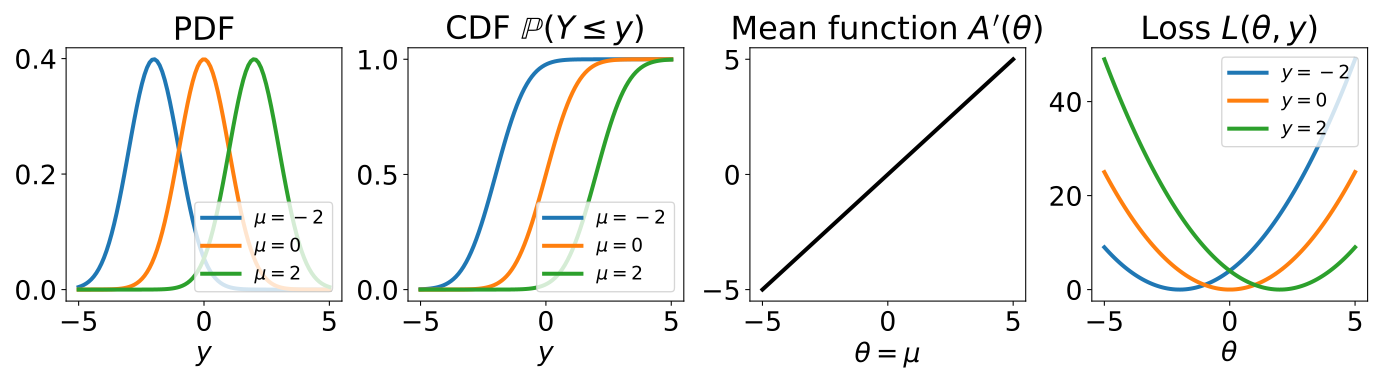
图 3.3:高斯分布,均值参数为 μ\mu,方差为 σ2=1\sigma^{2}=1。其均值函数为 μ=A′(θ)=θ\mu=A^{\prime}(\theta)=\theta,其中 θ\theta 例如是神经网络的输出。负对数似然导出平方损失 L(θ,y)=(y−θ)2L(\theta,y)=(y-\theta)^{2}。图中给出了 y∈{−2,0,2}y\in\{-2,0,2\} 下的损失曲线。Figure 3.3: The Gaussian distribution, with mean parameter μ\mu and variance σ2=1\sigma^{2}=1. Its mean function is μ=A′(θ)=θ\mu=A^{\prime}(\theta)=\theta, where θ\theta is for instance the output of a neural network. The negative log-likelihood leads to the squared loss, L(θ,y)=(y−θ)2L(\theta,y)=(y-\theta)^{2}. The loss curve is shown for y∈{−2,0,2}y\in\{-2,0,2\}.

参数化Parameterization

回归中通常由模型输出均值,而标准差 σ\sigma 保持固定(一般设为 11)。由于 μ\mu 不受约束,我们可以直接令Typically, in regression, the mean is output by a model, while the standard deviation σ\sigma is kept fixed (typically set to 11). Since μ\mu is unconstrained, we can simply set

μ:=f(x,w)∈R,\mu\coloneqq f({\bm{x}},{\bm{w}})\in\mathbb{R},

其中 f ⁣:X×W→Rf\colon\mathcal{X}\times\mathcal{W}\to\mathbb{R} 例如是一个神经网络。也就是说,ff 的输出即为该分布的均值,where f ⁣:X×W→Rf\colon\mathcal{X}\times\mathcal{W}\to\mathbb{R} is for example a neural network. That is, the output of ff is the mean of the distribution,

EY∼pμ,1[Y]=μ=f(x,w).\mathbb{E}_{Y\sim p_{\mu,1}}[Y]=\mu=f({\bm{x}},{\bm{w}}).

我们也可以用 μ\mu 预测 P(Y≤y)\mathbb{P}(Y\leq y) 或 P(a<Y≤b)\mathbb{P}(a<Y\leq b),如上所示。We can also use μ\mu to predict P(Y≤y)\mathbb{P}(Y\leq y) or P(a<Y≤b)\mathbb{P}(a<Y\leq b), as shown above.

3.3.6 多元回归Multivariate regression

更一般地,对于多变量结果,其中 Y=RM\mathcal{Y}=\mathbb{R}^{M},我们可以采用如下参数的多元正态分布:More generally, for multivariate outcomes, where Y=RM\mathcal{Y}=\mathbb{R}^{M}, we can use a multivariate normal distribution with parameters

λ:=(μ,Σ),{\bm{\lambda}}\coloneqq({\bm{\mu}},{\bm{\Sigma}}),

其中 μ∈RM{\bm{\mu}}\in\mathbb{R}^{M} 为均值,Σ∈RM×M{\bm{\Sigma}}\in\mathbb{R}^{M\times M} 为协方差矩阵。若 YY 服从参数为 (μ,Σ)({\bm{\mu}},{\bm{\Sigma}}) 的多元正态分布,则记作where μ∈RM{\bm{\mu}}\in\mathbb{R}^{M} is the mean and Σ∈RM×M{\bm{\Sigma}}\in\mathbb{R}^{M\times M} is the covariance matrix. When YY follows a multivariate normal distribution with parameters (μ,Σ)({\bm{\mu}},{\bm{\Sigma}}), we write

Y∼Normal(μ,Σ).Y\sim\mathrm{Normal}({\bm{\mu}},{\bm{\Sigma}}).

概率密度函数为The PDF is

pμ,Σ(y):=1(2π)M∣Σ∣exp⁡(−12⟨y−μ,Σ−1(y−μ)⟩).p_{{\bm{\mu}},{\bm{\Sigma}}}({\bm{y}})\coloneqq\frac{1}{\sqrt{(2\pi)^{M}|{\bm{\Sigma}}|}}\exp\left(-\frac{1}{2}\langle{\bm{y}}-{\bm{\mu}},{\bm{\Sigma}}^{-1}({\bm{y}}-{\bm{\mu}})\rangle\right).

使用对角协方差矩阵,等价于对每个 YjY_{j} 分别使用 MM 个独立的正态分布,其中 j∈[M]j\in[M]。其期望为Using a diagonal covariance matrix is equivalent to using MM independent normal distributions for each YjY_{j}, for j∈[M]j\in[M]. The expectation is

EY∼pμ,Σ[Y]=μ.\mathbb{E}_{Y\sim p_{{\bm{\mu}},{\bm{\Sigma}}}}[Y]={\bm{\mu}}.

参数化Parameterization

通常,在多元回归中,均值由模型输出,而协方差矩阵保持固定(通常设为单位矩阵)。由于 μ{\bm{\mu}} 同样不受约束,我们只需令Typically, in multivariate regression, the mean is output by a model, while the covariance matrix is kept fixed (typically set to the identity matrix). Since μ{\bm{\mu}} is again unconstrained, we can simply set

μ:=f(x,w)∈RM.{\bm{\mu}}\coloneqq f({\bm{x}},{\bm{w}})\in\mathbb{R}^{M}.

更一般地,我们可以参数化函数 ff,使其同时输出均值 μ{\bm{\mu}} 和协方差矩阵 Σ{\bm{\Sigma}},即More generally, we can parametrize the function ff so as to output both the mean μ{\bm{\mu}} and the covariance matrix Σ{\bm{\Sigma}}, i.e.,

(μ,Σ):=f(x,w)∈RM×RM×M.({\bm{\mu}},{\bm{\Sigma}})\coloneqq f({\bm{x}},{\bm{w}})\in\mathbb{R}^{M}\times\mathbb{R}^{M\times M}.

函数 ff 的设计必须保证 Σ{\bm{\Sigma}} 对称且半正定。这一点很容易实现,例如,可对某个矩阵 S{\bm{S}} 参数化 Σ=SS⊤{\bm{\Sigma}}={\bm{S}}{\bm{S}}^{\top}。The function ff must be designed such that Σ{\bm{\Sigma}} is symmetric and positive semi-definite. This is easy to achieve for instance by parametrizing Σ=SS⊤{\bm{\Sigma}}={\bm{S}}{\bm{S}}^{\top} for some matrix S{\bm{S}}.

3.3.7 整数回归Integer regression

对于取值为整数的结果,即 Y=N\mathcal{Y}=\mathbb{N},我们可以选用均值参数为 λ>0\lambda>0 的 Poisson 分布,当然也可作其他选择。当 YY 服从参数为 λ\lambda 的 Poisson 分布时,我们记作For integer outcomes, where Y=N\mathcal{Y}=\mathbb{N}, we can use, among other choices, a Poisson distribution with mean parameter λ>0\lambda>0. When YY follows a Poisson distribution with parameter λ\lambda, we write

Y∼Poisson(λ).Y\sim\mathrm{Poisson}(\lambda).

其概率质量函数为The PMF is

P(Y=y)=pλ(y):=λyexp⁡(−λ)y!.\mathbb{P}(Y=y)=p_{\lambda}(y)\coloneqq\frac{\lambda^{y}\exp(-\lambda)}{y!}.

它表示在一段时间区间内发生 yy 个事件的概率。当可能事件数量很大、而每个事件都很罕见时,常使用 Poisson 分布。It is the probability of yy events occurring in an interval of time. The Poisson distribution is frequently used when there is a large number of possible events, each of which is rare.

其累积分布函数为The CDF is

P(Y≤y)=∑i=0yP(Y=i).\mathbb{P}(Y\leq y)=\sum_{i=0}^{y}\mathbb{P}(Y=i).

Poisson 分布意味着离散指数(方差与均值之比)为 11,因为The Poisson distribution implies that the index of dispersion (the ratio between variance and mean) is 11, since

E[Y]=V[Y]=λ.\mathbb{E}[Y]=\mathbb{V}[Y]=\lambda.

当这一假设不再适用时,可以使用广义 Poisson 分布 [176]。When this assumption is inappropriate, one can use generalized Poisson distributions [176].
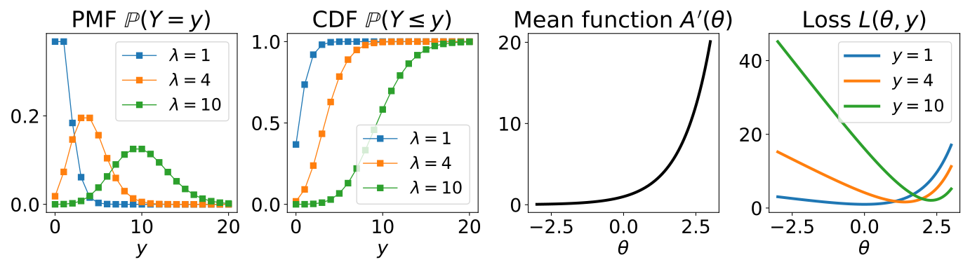
图 3.4:Poisson 分布,均值参数为 λ\lambda。对于概率质量函数和累积分布函数,标记之间的连线只为便于观察:Poisson 分布不会给非整数值分配概率质量。其均值函数为 λ=A′(θ)=exp⁡(θ)\lambda=A^{\prime}(\theta)=\exp(\theta),其中 θ\theta 例如是神经网络的输出。负对数似然导出 Poisson 损失 L(θ,y)=−log⁡pλ(y)=−yθ+exp⁡(θ)+log⁡(y!)L(\theta,y)=-\log p_{\lambda}(y)=-y\theta+\exp(\theta)+\log(y!),它是 θ\theta 的凸函数。损失曲线针对 y∈{1,4,10}y\in\{1,4,10\} 绘出。Figure 3.4: The Poisson distribution, with mean parameter λ\lambda. For the PMF and the CDF, the lines between markers are shown for visual aid: the Poisson distribution does not assign probability mass to non-integer values. Its mean function is λ=A′(θ)=exp⁡(θ)\lambda=A^{\prime}(\theta)=\exp(\theta), where θ\theta is for instance the output of a neural network. The negative log-likelihood leads to the Poisson loss, L(θ,y)=−log⁡pλ(y)=−yθ+exp⁡(θ)+log⁡(y!)L(\theta,y)=-\log p_{\lambda}(y)=-y\theta+\exp(\theta)+\log(y!), which is a convex function of θ\theta. The loss curve is shown for y∈{1,4,10}y\in\{1,4,10\}.

使用指数函数进行参数化Parameterization using an exponential

由于 Poisson 分布的参数 λ\lambda 必须严格为正,我们通常使用指数函数作为输出层:Since the parameter λ\lambda of a Poisson distribution needs to be strictly positive, we typically use an exponential function as output layer:

λ:=f(x,w):=exp⁡(g(x,w))>0,\lambda\coloneqq f({\bm{x}},{\bm{w}})\coloneqq\exp(g({\bm{x}},{\bm{w}}))>0,

其中 g ⁣:X×W→Rg\colon\mathcal{X}\times\mathcal{W}\to\mathbb{R}。where g ⁣:X×W→Rg\colon\mathcal{X}\times\mathcal{W}\to\mathbb{R}.

3.3.8 损失函数Loss functions

下面讨论如何从输入—输出对 (x1,y1),…,(xN,yN)({\bm{x}}_{1},{\bm{y}}_{1}),\dots,({\bm{x}}_{N},{\bm{y}}_{N}) 中学习模型参数 w∈W{\bm{w}}\in\mathcal{W}。We now discuss how to learn the model parameters w∈W{\bm{w}}\in\mathcal{W} from input-output pairs (x1,y1),…,(xN,yN)({\bm{x}}_{1},{\bm{y}}_{1}),\dots,({\bm{x}}_{N},{\bm{y}}_{N}).

确定性方法与概率方法Deterministic vs. probabilistic approaches

在确定性方法中,若采用映射 f ⁣:X×W→Yf\colon\mathcal{X}\times\mathcal{W}\to\mathcal{Y},我们可以构造如下形式的目标函数In a deterministic approach, if we used a mapping f ⁣:X×W→Yf\colon\mathcal{X}\times\mathcal{W}\to\mathcal{Y}, we could formulate an objective function of the form

L(w):=1N∑i=1Nℓ(f(xi,w),yi),L({\bm{w}})\coloneqq\frac{1}{N}\sum_{i=1}^{N}\ell(f({\bm{x}}_{i},{\bm{w}}),{\bm{y}}_{i}),

其中 ℓ ⁣:Y×Y→R\ell\colon\mathcal{Y}\times\mathcal{Y}\to\mathbb{R} 是损失函数。遗憾的是,若 Y\mathcal{Y} 是离散输出空间(分类情形即如此),则 L(w)L({\bm{w}}) 通常是不连续的,从而令优化变得困难。where ℓ ⁣:Y×Y→R\ell\colon\mathcal{Y}\times\mathcal{Y}\to\mathbb{R} is a loss function. Unfortunately, L(w)L({\bm{w}}) would be typically discontinuous if Y\mathcal{Y} is a discrete output space (as is the case in classification), making optimization difficult.

相比之下,在概率方法中,我们用映射 f ⁣:X×W→Λf\colon\mathcal{X}\times\mathcal{W}\to\Lambda 得到分布参数,并可构造如下形式的目标:In contrast, in the probabilistic approach, we use a mapping f ⁣:X×W→Λf\colon\mathcal{X}\times\mathcal{W}\to\Lambda to distribution parameters, and we can formulate an objective of the form

L(w):=1N∑i=1Nℓ(f(xi,w),yi),L({\bm{w}})\coloneqq\frac{1}{N}\sum_{i=1}^{N}\ell(f({\bm{x}}_{i},{\bm{w}}),{\bm{y}}_{i}),

其中 ℓ ⁣:Λ×Y→R\ell\colon\Lambda\times\mathcal{Y}\to\mathbb{R}。这通常是连续目标,因为 Λ\Lambda 通常是连续集,且即便 pλp_{\bm{\lambda}} 是离散集 Y\mathcal{Y} 上的分布,pλp_{\bm{\lambda}} 也会关于 λ{\bm{\lambda}} 连续变化。换言之,概率方法之所以强大,不仅在于它允许我们进行推断(概率、期望、方差、众数),还在于它允许我们构造连续且通常可微的目标函数!where ℓ ⁣:Λ×Y→R\ell\colon\Lambda\times\mathcal{Y}\to\mathbb{R}. This is typically a continuous objective, since Λ\Lambda is typically a continuous set and pλp_{\bm{\lambda}} varies continuously w.r.t. λ{\bm{\lambda}} even if pλp_{\bm{\lambda}} is a distribution over a discrete set Y\mathcal{Y}. In other words, the probabilistic approach is not only powerful for the inference it allows us to do (probability, expectation, variance, mode), but also because it allows us to formulate a continuous and typically differentiable objective function!

图 3.5 对此进行了总结。This is summarized in Fig. 3.5.
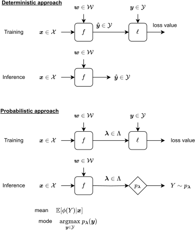
图 3.5:确定性方法与概率方法的总结。Figure 3.5: Summary of deterministic vs. probabilistic approaches.

负对数似然Negative log-likelihood

在 3.3.1 节简要回顾的条件设定下,我们可以使用最大似然估计(MLE)来估计 ff 的模型参数 w∈W{\bm{w}}\in\mathcal{W}。给定一组输入—输出对 (x1,y1),…,(xN,yN)({\bm{x}}_{1},{\bm{y}}_{1}),\dots,({\bm{x}}_{N},{\bm{y}}_{N}),我们选取使数据似然最大化的模型参数,In the conditional setting briefly reviewed in Section 3.3.1, we can use maximum likelihood estimation (MLE) to estimate the model parameters w∈W{\bm{w}}\in\mathcal{W} of ff. Given a set of input-output pairs (x1,y1),…,(xN,yN)({\bm{x}}_{1},{\bm{y}}_{1}),\dots,({\bm{x}}_{N},{\bm{y}}_{N}), we choose the model parameters that maximize the likelihood of the data,

w^N:=arg max⁡w∈W∏i=1Npλi(yi),\widehat{\bm{w}}_{N}\coloneqq\argmax_{{\bm{w}}\in\mathcal{W}}\prod_{i=1}^{N}p_{{\bm{\lambda}}_{i}}({\bm{y}}_{i}),

其中where

λi:=f(xi,w).{\bm{\lambda}}_{i}\coloneqq f({\bm{x}}_{i},{\bm{w}}).

同样,这等价于最小化负对数似然,Again, this is equivalent to minimizing the negative log-likelihood,

w^N=arg min⁡w∈W−∑i=1Nlog⁡pλi(yi).\widehat{\bm{w}}_{N}=\argmin_{{\bm{w}}\in\mathcal{W}}-\sum_{i=1}^{N}\log p_{{\bm{\lambda}}_{i}}({\bm{y}}_{i}).

在上述记号下,这对应于定义如下损失函数:In the notation above, this corresponds to defining the loss function

ℓ(λi,yi):=−log⁡pλi(yi).\ell({\bm{\lambda}}_{i},{\bm{y}}_{i})\coloneqq-\log p_{{\bm{\lambda}}_{i}}({\bm{y}}_{i}).

恢复出众所周知的损失函数。Recovering well-known loss functions

有趣的是,MLE 使我们能够推导出若干流行的损失函数。Interestingly, MLE allows us to recover several popular loss functions.

  • •

    对于参数为 λi=πi=logistic(θi)\lambda_{i}=\pi_{i}=\mathrm{logistic}(\theta_{i}) 的 伯努利分布,其中 θi:=g(xi,w)\theta_{i}\coloneqq g({\bm{x}}_{i},{\bm{w}}),我们有For the Bernoulli distribution with parameter λi=πi=logistic(θi)\lambda_{i}=\pi_{i}=\mathrm{logistic}(\theta_{i}), where θi:=g(xi,w)\theta_{i}\coloneqq g({\bm{x}}_{i},{\bm{w}}), we have

    −log⁡pλi(yi)\displaystyle-\log p_{\lambda_{i}}(y_{i}) =−[yilog⁡πi+(1−yi)log⁡(1−πi)]\displaystyle=-\left[y_{i}\log\pi_{i}+(1-y_{i})\log(1-\pi_{i})\right]
    =log⁡(1+exp⁡(θi))−yiθi\displaystyle=\log(1+\exp(\theta_{i}))-y_{i}\theta_{i}
    =softplus(θi)−yiθi,\displaystyle=\mathrm{softplus}(\theta_{i})-y_{i}\theta_{i},

    即二分类 logistic 损失函数。which is the binary logistic loss function.

  • •

    对于参数为 λi=πi=softargmax(θi){\bm{\lambda}}_{i}={\bm{\pi}}_{i}=\mathrm{softargmax}({\bm{\theta}}_{i}) 的 分类分布,其中 θi:=g(xi,w){\bm{\theta}}_{i}\coloneqq g({\bm{x}}_{i},{\bm{w}}),我们有For the categorical distribution with parameters λi=πi=softargmax(θi){\bm{\lambda}}_{i}={\bm{\pi}}_{i}=\mathrm{softargmax}({\bm{\theta}}_{i}), where θi:=g(xi,w){\bm{\theta}}_{i}\coloneqq g({\bm{x}}_{i},{\bm{w}}), we have

    −log⁡pλi(yi)\displaystyle-\log p_{{\bm{\lambda}}_{i}}(y_{i}) =−log⁡πi,yi\displaystyle=-\log\pi_{i,y_{i}}
    =log⁡∑j=1Mexp⁡(θi,j)−θi,yi\displaystyle=\log\sum_{j=1}^{M}\exp(\theta_{i,j})-\theta_{i,y_{i}}
    =logsumexp(θi)−⟨θi,eyi⟩,\displaystyle=\mathrm{logsumexp}({\bm{\theta}}_{i})-\langle{\bm{\theta}}_{i},{\bm{e}}_{y_{i}}\rangle,

    即多分类 logistic 损失函数,也称为交叉熵损失。which is the multiclass logistic loss function, also known as cross-entropy loss.

  • •

    对于均值为 λi=μi=f(xi,w)\lambda_{i}=\mu_{i}=f({\bm{x}}_{i},{\bm{w}})、方差固定为 σi2\sigma_{i}^{2} 的正态分布,我们有For the normal distribution with mean λi=μi=f(xi,w)\lambda_{i}=\mu_{i}=f({\bm{x}}_{i},{\bm{w}}) and fixed variance σi2\sigma_{i}^{2}, we have

    −log⁡pλi(yi)=12σi2(yi−μi)2+12log⁡σi2+12log⁡(2π),-\log p_{\lambda_{i}}(y_{i})=\frac{1}{2\sigma_{i}^{2}}(y_{i}-\mu_{i})^{2}+\frac{1}{2}\log\sigma_{i}^{2}+\frac{1}{2}\log(2\pi),

    在相差一个常数且方差为单位方差的意义下,这就是平方损失函数。which is, up to a constant and with unit variance, the squared loss function.

  • •

    对于均值为 λi=exp⁡(θi)\lambda_{i}=\exp(\theta_{i}) 的 Poisson 分布,其中 θi:=g(xi,w)\theta_{i}\coloneqq g({\bm{x}}_{i},{\bm{w}}),我们有For the Poisson distribution with mean λi=exp⁡(θi)\lambda_{i}=\exp(\theta_{i}), where θi:=g(xi,w)\theta_{i}\coloneqq g({\bm{x}}_{i},{\bm{w}}), we have

    −log⁡pλi(yi)\displaystyle-\log p_{\lambda_{i}}(y_{i}) =−yilog⁡(λi)+λi+log⁡(yi!)\displaystyle=-y_{i}\log(\lambda_{i})+\lambda_{i}+\log(y_{i}!)
    =−yiθi+exp⁡(θi)+log⁡(yi!)\displaystyle=-y_{i}\theta_{i}+\exp(\theta_{i})+\log(y_{i}!)

    即 Poisson 损失函数。对于 yi≥0y_{i}\geq 0,该损失函数关于 λi\lambda_{i} 与 θi\theta_{i} 是凸的。which is the Poisson loss function. The loss function is convex w.r.t. λi\lambda_{i} and θi\theta_{i} for yi≥0y_{i}\geq 0.

3.4 指数族分布3.4 Exponential family distributions

3.4.1 定义Definition

指数族是一类概率分布,其 PMF 或 PDF 可以写成如下形式:The exponential family is a class of probability distributions, whose PMF or PDF can be written in the form

pθ(y)\displaystyle p_{\bm{\theta}}({\bm{y}}) =h(y)exp⁡[⟨θ,ϕ(y)⟩]exp⁡(A(θ))\displaystyle=\frac{h({\bm{y}})\exp\left[\langle{\bm{\theta}},\phi({\bm{y}})\rangle\right]}{\exp(A({\bm{\theta}}))}
=h(y)exp⁡[⟨θ,ϕ(y)⟩−A(θ)],\displaystyle=h({\bm{y}})\exp\left[\langle{\bm{\theta}},\phi({\bm{y}})\rangle-A({\bm{\theta}})\right],

其中 θ{\bm{\theta}} 是分布的自然参数或典范参数。函数 hh 称为基测度;函数 ϕ\phi 为充分统计量,它承载了关于 y{\bm{y}} 的全部信息,并用于将 y{\bm{y}} 嵌入向量空间。函数 AA 称为对数配分函数或对数归一化函数(详见下文)。我们在 3.3 节中回顾的所有分布均属于指数族。这里我们略微滥用了记号:以 pλp_{\bm{\lambda}} 表示原始形式的分布,以 pθp_{\bm{\theta}} 表示指数族形式的分布。正如我们将看到的,由 θ{\bm{\theta}} 可得 λ{\bm{\lambda}},反之亦然。下文将说明如何将分布改写为指数族形式。where θ{\bm{\theta}} are the natural or canonical parameters of the distribution. The function hh is known as the base measure. The function ϕ\phi is the sufficient statistic: it holds all the information about y{\bm{y}} and is used to embed y{\bm{y}} in a vector space. The function AA is the log-partition or log-normalizer (see below for details). All the distributions we reviewed in Section 3.3 belong to the exponential family. With some abuse of notation, we use pλp_{\bm{\lambda}} for the distribution in original form and pθp_{\bm{\theta}} for the distribution in exponential family form. As we will see, we can go from θ{\bm{\theta}} to λ{\bm{\lambda}} and vice versa. We illustrate how to rewrite a distribution in exponential family form below.

例 3.4.1(伯努利分布)。Example 3.4.1 (Bernoulli distribution).
参数为 λ=π\lambda=\pi 的 伯努利分布,其 PMF 等于The PMF of the Bernoulli distribution with parameter λ=π\lambda=\pi equals pλ(y)\displaystyle p_{\lambda}(y) :=πy(1−π)1−y\displaystyle\coloneqq\pi^{y}(1-\pi)^{1-y} =exp⁡(log⁡(πy(1−π)1−y))\displaystyle=\exp(\log(\pi^{y}(1-\pi)^{1-y})) =exp⁡(ylog⁡(π)+(1−y)log⁡(1−π))\displaystyle=\exp(y\log(\pi)+(1-y)\log(1-\pi)) =exp⁡(log⁡(π/(1−π))y+log⁡(1−π))\displaystyle=\exp(\log(\pi/(1-\pi))y+\log(1-\pi)) =exp⁡(θy−log⁡(1+exp⁡(θ)))\displaystyle=\exp(\theta y-\log(1+\exp(\theta))) =exp⁡(θy−softplus(θ))\displaystyle=\exp(\theta y-\mathrm{softplus}(\theta)) =:pθ(y).\displaystyle\eqqcolon p_{\theta}(y). 因此,伯努利分布属于指数族,其自然参数为 θ=logit(π):=log⁡(π/(1+π))\theta=\mathrm{logit}(\pi)\coloneqq\log(\pi/(1+\pi))。反之,我们有 π=logistic(θ)=11+exp⁡(−θ)\pi=\mathrm{logistic}(\theta)=\frac{1}{1+\exp(-\theta)}。Therefore, Bernoulli distributions belong to the exponential family, with natural parameter θ=logit(π):=log⁡(π/(1+π))\theta=\mathrm{logit}(\pi)\coloneqq\log(\pi/(1+\pi)). Conversely, we have π=logistic(θ)=11+exp⁡(−θ)\pi=\mathrm{logistic}(\theta)=\frac{1}{1+\exp(-\theta)}.

表 3.1 将前述各分布改写为指数族形式。该列表并不详尽:指数族中的分布远不止这些![11]We rewrite the previously-described distributions in exponential family form in Table 3.1. This list is non-exhaustive: there are many more distributions in the exponential family! [11]

表 3.1:指数族分布示例。Table 3.1: Examples of distributions in the exponential family.
BernoulliBernoulli CategoricalCategorical
Y\mathcal{Y} {0,1}\{0,1\} [M][M]
λ{\bm{\lambda}} π=logistic(θ)\pi=\mathrm{logistic}(\theta) π=softargmax(θ){\bm{\pi}}=\mathrm{softargmax}({\bm{\theta}})
θ{\bm{\theta}} logit(π)\mathrm{logit}(\pi) log⁡π+A(θ)\log{\bm{\pi}}+A({\bm{\theta}})
ϕ(y)\phi(y) yy ey{\bm{e}}_{y}
A(θ)A({\bm{\theta}}) softplus(θ)\mathrm{softplus}(\theta) logsumexp(θ)\mathrm{logsumexp}({\bm{\theta}})
h(y)h(y) 1 1
正态分布(仅位置)Normal (location only) 正态分布(位置—尺度)Normal (location-scale)
Y\mathcal{Y} R\mathbb{R} R\mathbb{R}
λ{\bm{\lambda}} μ=θσ\mu=\theta\sigma (μ,σ2)=(−θ12θ2,−12θ2)(\mu,\sigma^{2})=(\frac{-\theta_{1}}{2\theta_{2}},\frac{-1}{2\theta_{2}})
θ{\bm{\theta}} μσ\frac{\mu}{\sigma} (μσ2,−12σ2)(\frac{\mu}{\sigma^{2}},\frac{-1}{2\sigma^{2}})
ϕ(y)\phi(y) yσ\frac{y}{\sigma} (y,y2)(y,y^{2})
A(θ)A({\bm{\theta}}) θ22=μ22σ2\frac{\theta^{2}}{2}=\frac{\mu^{2}}{2\sigma^{2}} −θ124θ2−12log⁡(−2θ2)=μ22σ2+log⁡σ\frac{-\theta_{1}^{2}}{4\theta_{2}}-\frac{1}{2}\log(-2\theta_{2})=\frac{\mu^{2}}{2\sigma^{2}}+\log\sigma
h(y)h(y) exp⁡(−y22σ2)2πσ\frac{\exp(\frac{-y^{2}}{2\sigma^{2}})}{\sqrt{2\pi}\sigma} 12π\frac{1}{\sqrt{2\pi}}
多元正态分布Multivariate normal PoissonPoisson
Y\mathcal{Y} RM\mathbb{R}^{M} N\mathbb{N}
λ{\bm{\lambda}} (μ,Σ)=(−12θ2−1θ1,−12θ2−1)({\bm{\mu}},{\bm{\Sigma}})=(-\frac{1}{2}{\bm{\theta}}_{2}^{-1}{\bm{\theta}}_{1},-\frac{1}{2}{\bm{\theta}}_{2}^{-1}) λ=exp⁡(θ)\lambda=\exp(\theta)
θ{\bm{\theta}} (Σ−1μ,−12Σ−1)({\bm{\Sigma}}^{-1}{\bm{\mu}},-\frac{1}{2}{\bm{\Sigma}}^{-1}) log⁡λ\log\lambda
ϕ(y)\phi({\bm{y}}) (y,yy⊤)({\bm{y}},{\bm{y}}{\bm{y}}^{\top}) yy
A(θ)A({\bm{\theta}}) −14θ1⊤θ2−1θ1−12log⁡∣−2θ2∣-\frac{1}{4}{\bm{\theta}}_{1}^{\top}{\bm{\theta}}_{2}^{-1}{\bm{\theta}}_{1}-\frac{1}{2}\log|-2{\bm{\theta}}_{2}| exp⁡(θ)\exp(\theta)
=12μ⊤Σ−1μ+12log⁡∣Σ∣=\frac{1}{2}{\bm{\mu}}^{\top}{\bm{\Sigma}}^{-1}{\bm{\mu}}+\frac{1}{2}\log|{\bm{\Sigma}}|
h(y)h({\bm{y}}) (2π)−M/2(2\pi)^{-M/2} 1/y!1/y!

3.4.2 对数配分函数The log-partition function

为简明起见,本节讨论集中于离散变量。不过,本节所述结果对连续变量同样成立 [206]。对数配分函数 AA 即分布归一化因子的对数,We focus our discussion in this section on discrete variables for simplicity. However, the results stated in this section also hold for continuous variables [206]. The log-partition function AA is the logarithm of the distribution’s normalization factor,

A(θ):=log⁡∑y∈Yh(y)exp⁡[⟨θ,ϕ(y)⟩].A({\bm{\theta}})\coloneqq\log\sum_{{\bm{y}}\in\mathcal{Y}}h({\bm{y}})\exp\left[\langle{\bm{\theta}},\phi({\bm{y}})\rangle\right].

我们记有效参数集为We denote the set of valid parameters

Θ:={θ∈RM ⁣:A(θ)<+∞}⊆RM.\Theta\coloneqq\{{\bm{\theta}}\in\mathbb{R}^{M}\colon A({\bm{\theta}})<+\infty\}\subseteq\mathbb{R}^{M}.

可方便地将 A(θ)A({\bm{\theta}}) 改写为We can conveniently rewrite A(θ)A({\bm{\theta}}) as

A(θ)=logsumexp(B(θ)):=log⁡∑y∈Yexp⁡([B(θ)]y),A({\bm{\theta}})=\mathrm{logsumexp}(B({\bm{\theta}}))\coloneqq\log\sum_{{\bm{y}}\in\mathcal{Y}}\exp([B({\bm{\theta}})]_{\bm{y}}),

其中定义了仿射映射where we defined the affine map

B(θ):=(⟨θ,ϕ(y)⟩+log⁡h(y))y∈Y.B({\bm{\theta}})\coloneqq(\langle{\bm{\theta}},\phi({\bm{y}})\rangle+\log h({\bm{y}}))_{{\bm{y}}\in\mathcal{Y}}.

由于 A(θ)A({\bm{\theta}}) 是凸函数 logsumexp\mathrm{logsumexp} 与仿射映射 BB 的复合,我们立即可得如下命题。Since A(θ)A({\bm{\theta}}) is the composition of logsumexp\mathrm{logsumexp}, a convex function, and of BB, an affine map, we immediately obtain the following proposition.

命题 3.4.2(对数配分函数的凸性)。Proposition 3.4.2 (Convexity of the log-partition).
A(θ)A({\bm{\theta}}) 是一个凸函数。A(θ)A({\bm{\theta}}) is a convex function.

对数配分函数的一个主要性质是:其梯度等于 ϕ(Y)\phi(Y) 在 pθp_{\bm{\theta}} 下的期望。A major property of the log-partition function is that its gradient coincides with the expectation of ϕ(Y)\phi(Y) according to pθp_{\bm{\theta}}.

命题 3.4.3(对数配分函数的梯度)。Proposition 3.4.3 (Gradient of the log-partition).
μ(θ):=∇A(θ)=EY∼pθ[ϕ(Y)]∈M.\displaystyle{\bm{\mu}}({\bm{\theta}})\coloneqq\nabla A({\bm{\theta}})=\mathbb{E}_{Y\sim p_{\bm{\theta}}}[\phi(Y)]\in\mathcal{M}.
证明 3.4.4。Proof 3.4.4.

该结果直接由下式得出The result follows directly from

∇A(θ)=∂B(θ)∗∇logsumexp(B(θ))=(ϕ(y))y∈Y softmax(B(θ)).\nabla A({\bm{\theta}})=\partial B({\bm{\theta}})^{*}\nabla\mathrm{logsumexp}(B({\bm{\theta}}))=(\phi({\bm{y}}))_{{\bm{y}}\in\mathcal{Y}} \ \mathrm{softmax}(B({\bm{\theta}})).

因此,梯度 ∇A(θ)\nabla A({\bm{\theta}}) 常被称为均值函数。可达均值的集合 μ(θ){\bm{\mu}}({\bm{\theta}}) 定义为The gradient ∇A(θ)\nabla A({\bm{\theta}}) is therefore often called the mean function. The set of achievable means μ(θ){\bm{\mu}}({\bm{\theta}}) is defined by

M:=conv(ϕ(Y)):={Ep[ϕ(Y)] ⁣:p∈P(Y)},\mathcal{M}\coloneqq\mathrm{conv}(\phi(\mathcal{Y}))\coloneqq\{\mathbb{E}_{p}[\phi(Y)]\colon p\in\mathcal{P}(\mathcal{Y})\},

其中 conv(S)\mathrm{conv}(\mathcal{S}) 为 S\mathcal{S} 的凸包,P(Y)\mathcal{P}(\mathcal{Y}) 为 Y\mathcal{Y} 上有效概率分布的集合。where conv(S)\mathrm{conv}(\mathcal{S}) is the convex hull of S\mathcal{S} and P(Y)\mathcal{P}(\mathcal{Y}) is the set of valid probability distributions over Y\mathcal{Y}.

类似地,Hessian 矩阵 ∇2A(θ)\nabla^{2}A({\bm{\theta}}) 等于 ϕ(Y)\phi(Y) 在 pθp_{\bm{\theta}} 下的协方差矩阵 [206,第 3 章]。Similarly, the Hessian ∇2A(θ)\nabla^{2}A({\bm{\theta}}) coincides with the covariance matrix of ϕ(Y)\phi(Y) according to pθp_{\bm{\theta}} [206, Chapter 3].

当指数族为极小指数族,即参数 θ{\bm{\theta}} 能够唯一确定分布时,已知 ∇A\nabla A 是从 Θ\Theta 到 M\mathcal{M} 的一一映射。也就是说,μ(θ)=∇A(θ){\bm{\mu}}({\bm{\theta}})=\nabla A({\bm{\theta}}) 且 θ=(∇A)−1(μ(θ)){\bm{\theta}}=(\nabla A)^{-1}({\bm{\mu}}({\bm{\theta}}))。When the exponential family is minimal, which means that the parameters θ{\bm{\theta}} uniquely identify the distribution, it is known that ∇A\nabla A is a one-to-one mapping from Θ\Theta to M\mathcal{M}. That is, μ(θ)=∇A(θ){\bm{\mu}}({\bm{\theta}})=\nabla A({\bm{\theta}}) and θ=(∇A)−1(μ(θ)){\bm{\theta}}=(\nabla A)^{-1}({\bm{\mu}}({\bm{\theta}})).

3.4.3 最大熵原理Maximum entropy principle

假设我们观测到若干观测值 y1,…,yN{\bm{y}}_{1},\dots,{\bm{y}}_{N} 的经验均值 μ^=1N∑i=1Nϕ(yi)∈M\widehat{\bm{\mu}}=\frac{1}{N}\sum_{i=1}^{N}\phi({\bm{y}}_{i})\in\mathcal{M}。如何找到一个能达到该均值的概率分布?显然,这样的分布未必唯一。在所有可能的分布中做出选择,一种办法是运用最大熵原理。我们将 Shannon 熵定义为Suppose we observe the empirical mean μ^=1N∑i=1Nϕ(yi)∈M\widehat{\bm{\mu}}=\frac{1}{N}\sum_{i=1}^{N}\phi({\bm{y}}_{i})\in\mathcal{M} of some observations y1,…,yN{\bm{y}}_{1},\dots,{\bm{y}}_{N}. How do we find a probability distribution achieving this mean? Clearly, such a distribution may not be unique. One way to choose among all possible distributions is by using the maximum entropy principle. Let us define the Shannon entropy by

H(p):=−∑y∈Yp(y)log⁡p(y)H(p)\coloneqq-\sum_{{\bm{y}}\in\mathcal{Y}}p({\bm{y}})\log p({\bm{y}})

对离散变量,以及通过for discrete variables and by

H(p):=−∫Yp(y)log⁡p(y)dyH(p)\coloneqq-\int_{\mathcal{Y}}p(y)\log p(y)dy

对连续变量。它刻画了 pp 中“不确定性”的高低,也就是说,分布为均匀分布时它取最大值。于是,满足一阶矩条件(即其期望与经验均值相符)的最大熵分布为for continuous variables. This captures the level of “uncertainty” in pp, i.e., it is maximized when the distribution is uniform. Then, the maximum entropy distribution satisfying the first-order moment condition (i.e., whose expectation matches the empirical mean) is

p⋆:=arg max⁡p∈P(Y)H(p)s.t.EY∼p[ϕ(Y)]=μ^.p^{\star}\coloneqq\argmax_{p\in\mathcal{P}(\mathcal{Y})}H(p)\quad\text{s.t.}\quad\mathbb{E}_{Y\sim p}[\phi(Y)]=\widehat{\bm{\mu}}.

可以证明,最大熵分布必然属于指数族,其充分统计量由 ϕ\phi 定义,而其典范参数 θ{\bm{\theta}} 与上述约束的拉格朗日乘子相一致 [206,第 3.1 节]。It can be shown that the maximum entropy distribution is necessarily in the exponential family with sufficient statistic defined by ϕ\phi and its canonical parameters θ{\bm{\theta}} coincide with the Lagrange multipliers of the above constraint [206, Section 3.1].

3.4.4 最大似然估计Maximum likelihood estimation

如同第 3.2 节,为了将指数族分布的参数 θ∈Θ{\bm{\theta}}\in\Theta 拟合到若干独立同分布的观测 y1,…,yN{\bm{y}}_{1},\dots,{\bm{y}}_{N},我们可以采用 MLE 原则,即As in Section 3.2, to fit the parameters θ∈Θ{\bm{\theta}}\in\Theta of an exponential family distribution to some i.i.d. observations y1,…,yN{\bm{y}}_{1},\dots,{\bm{y}}_{N}, we can use the MLE principle, i.e.,

θ^N=arg max⁡θ∈Θ∏i=1Npθ(yi)=arg min⁡θ∈Θ−∑i=1Nlog⁡pθ(yi).\widehat{\bm{\theta}}_{N}=\argmax_{{\bm{\theta}}\in\Theta}\prod_{i=1}^{N}p_{\bm{\theta}}({\bm{y}}_{i})=\argmin_{{\bm{\theta}}\in\Theta}-\sum_{i=1}^{N}\log p_{\bm{\theta}}({\bm{y}}_{i}).

所幸,对于指数族分布,对数概率/密度具有格外简单的形式。Fortunately, for exponential family distributions, the log probability/density enjoys a particularly simple form.

命题 3.4.5(负对数似然)。Proposition 3.4.5 (Negative log-likelihood).
指数族分布的负对数似然为The negative log-likelihood of an exponential family distribution is −log⁡pθ(y)=A(θ)−⟨θ,ϕ(y)⟩−log⁡h(y).-\log p_{\bm{\theta}}({\bm{y}})=A({\bm{\theta}})-\langle{\bm{\theta}},\phi({\bm{y}})\rangle-\log h({\bm{y}}). 其梯度为Its gradient is −∇θlog⁡pθ(y)=∇A(θ)−ϕ(y)=EY∼pθ[ϕ(Y)]−ϕ(y)-\nabla_{\bm{\theta}}\log p_{\bm{\theta}}({\bm{y}})=\nabla A({\bm{\theta}})-\phi({\bm{y}})=\mathbb{E}_{Y\sim p_{\bm{\theta}}}[\phi(Y)]-\phi({\bm{y}}) 其 Hessian 矩阵为and its Hessian is −∇θ2log⁡pθ(y)=∇2A(θ),-\nabla^{2}_{\bm{\theta}}\log p_{\bm{\theta}}({\bm{y}})=\nabla^{2}A({\bm{\theta}}), 它与 y{\bm{y}} 无关。which is independent of y{\bm{y}}.

由命题 3.4.2 可知 θ↦−log⁡pθ(y){\bm{\theta}}\mapsto-\log p_{\bm{\theta}}({\bm{y}}) 是凸的。有趣的是,这里的梯度正是模型下 ϕ(Y)\phi(Y) 的期望与观测到的 ϕ(y)\phi({\bm{y}}) 之间的残差。因此,指数族分布的负对数似然可以视为在进行一阶矩匹配。It follows from Proposition 3.4.2 that θ↦−log⁡pθ(y){\bm{\theta}}\mapsto-\log p_{\bm{\theta}}({\bm{y}}) is convex. Interestingly, we see that the gradient is the residual between the expectation of ϕ(Y)\phi(Y) according to the model and the observed ϕ(y)\phi({\bm{y}}). Therefore, the negative log-likelihood of an exponential family distribution can be seen as performing first moment matching.

3.4.5 使用指数族的概率学习Probabilistic learning with exponential families

在概率监督学习设定中,我们希望估计形如 pw(y∣x)p_{\bm{w}}({\bm{y}}\mid{\bm{x}}) 的条件分布。给定模型函数 ff(例如神经网络),定义这类条件分布的一种常见做法是将其归约为无条件设定,In the supervised probabilistic learning setting, we wish to estimate a conditional distribution of the form pw(y∣x)p_{\bm{w}}({\bm{y}}\mid{\bm{x}}). Given a model function ff, such as a neural network, a common approach for defining such a conditional distribution is by reduction to the unconditional setting,

pw(y∣x):=pθ(y)whereθ:=f(x,w).p_{\bm{w}}({\bm{y}}\mid{\bm{x}})\coloneqq p_{\bm{\theta}}({\bm{y}})\quad\text{where}\quad{\bm{\theta}}\coloneqq f({\bm{x}},{\bm{w}}).

换言之,ff 的作用是在给定某个输入 x{\bm{x}} 时产生 pθp_{\bm{\theta}} 的参数。它是从 X×W\mathcal{X}\times\mathcal{W} 到 Θ\Theta 的函数。注意,ff 的设计必须使其输出落在In other words, the role of ff is to produce the parameters of pθp_{\bm{\theta}} given some input x{\bm{x}}. It is a function from X×W\mathcal{X}\times\mathcal{W} to Θ\Theta. Note that ff must be designed such that it produces an output in

Θ:={θ∈RM ⁣:A(θ)<+∞}.\Theta\coloneqq\{{\bm{\theta}}\in\mathbb{R}^{M}\colon A({\bm{\theta}})<+\infty\}.

很多时候,Θ\Theta 就是整个 RM\mathbb{R}^{M},但情况并非总是如此。例如,正如前文所述,对于多元正态分布,当 θ=(μ,Σ)=f(x,w){\bm{\theta}}=({\bm{\mu}},{\bm{\Sigma}})=f({\bm{x}},{\bm{w}}) 时,我们需要确保 Σ{\bm{\Sigma}} 为半正定矩阵。Many times, Θ\Theta will be the entire RM\mathbb{R}^{M} but this is not always the case. For instance, as we previously discussed, for a multivariate normal distribution, where θ=(μ,Σ)=f(x,w){\bm{\theta}}=({\bm{\mu}},{\bm{\Sigma}})=f({\bm{x}},{\bm{w}}), we need to ensure that Σ{\bm{\Sigma}} is a positive semidefinite matrix.

训练Training

给定输入—输出对 {(xi,yi)}i=1N\{({\bm{x}}_{i},{\bm{y}}_{i})\}_{i=1}^{N},我们接下来通过最小化负对数似然,来求取 f(x,w)f({\bm{x}},{\bm{w}}) 的参数 w{\bm{w}}:Given input-output pairs {(xi,yi)}i=1N\{({\bm{x}}_{i},{\bm{y}}_{i})\}_{i=1}^{N}, we then seek to find the parameters w{\bm{w}} of f(x,w)f({\bm{x}},{\bm{w}}) by minimizing the negative log-likelihood

arg min⁡w∈W−∑i=1Nlog⁡pθi(yi)=arg min⁡w∈W∑i=1NA(θi)−⟨θi,ϕ(yi)⟩\argmin_{{\bm{w}}\in\mathcal{W}}-\sum_{i=1}^{N}\log p_{{\bm{\theta}}_{i}}({\bm{y}}_{i})=\argmin_{{\bm{w}}\in\mathcal{W}}\sum_{i=1}^{N}A({\bm{\theta}}_{i})-\langle{\bm{\theta}}_{i},\phi({\bm{y}}_{i})\rangle

其中 θi:=f(xi,w){\bm{\theta}}_{i}\coloneqq f({\bm{x}}_{i},{\bm{w}})。对于指数族分布,−log⁡pθ(y)-\log p_{\bm{\theta}}({\bm{y}}) 虽是 θ{\bm{\theta}} 的凸函数,但我们要强调:当 ff 为非线性函数(例如神经网络)时,−log⁡pf(x,w)(y)-\log p_{f({\bm{x}},{\bm{w}})}({\bm{y}}) 通常是 w{\bm{w}} 的非凸函数。where θi:=f(xi,w){\bm{\theta}}_{i}\coloneqq f({\bm{x}}_{i},{\bm{w}}). While −log⁡pθ(y)-\log p_{\bm{\theta}}({\bm{y}}) is a convex function of θ{\bm{\theta}} for exponential family distributions, we emphasize that −log⁡pf(x,w)(y)-\log p_{f({\bm{x}},{\bm{w}})}({\bm{y}}) is typically a nonconvex function of w{\bm{w}}, when ff is a nonlinear function, such as a neural network.
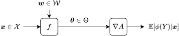
图 3.6:广义线性模型。Figure 3.6: Generalized linear models.

推断Inference

通过最小化上述目标函数求得 w{\bm{w}} 之后,我们可用若干策略对新输入 x{\bm{x}} 进行推断。Once we have found w{\bm{w}} by minimizing the objective function above, there are several possible strategies to perform inference for a new input x{\bm{x}}.

  • •

    期望。若目标是计算 ϕ(Y)\phi(Y) 的期望,可以使用 ∇A(f(x,w))\nabla A(f({\bm{x}},{\bm{w}}))。也就是说,先用 θ=f(x,w){\bm{\theta}}=f({\bm{x}},{\bm{w}}) 算出与 x{\bm{x}} 对应的分布参数,再用 μ=∇A(θ){\bm{\mu}}=\nabla A({\bm{\theta}}) 求出均值。当 ff 关于 w{\bm{w}} 为线性时,复合 ∇A∘f\nabla A\circ f 便称为广义线性模型。图 3.6 说明了这一点。Expectation. When the goal is to compute the expectation of ϕ(Y)\phi(Y), we can use ∇A(f(x,w))\nabla A(f({\bm{x}},{\bm{w}})). That is, we compute the distribution parameters associated with x{\bm{x}} by θ=f(x,w){\bm{\theta}}=f({\bm{x}},{\bm{w}}) and then we compute the mean by μ=∇A(θ){\bm{\mu}}=\nabla A({\bm{\theta}}). When ff is linear in w{\bm{w}}, the composition ∇A∘f\nabla A\circ f is called a generalized linear model. This is illustrated in Fig. 3.6.

  • •

    概率。若目标是计算某个 y{\bm{y}} 的概率,可以先用 θ=f(x,w){\bm{\theta}}=f({\bm{x}},{\bm{w}}) 算出与 x{\bm{x}} 对应的分布参数,再计算 P(Y=y∣X=x)=pθ(y)\mathbb{P}(Y={\bm{y}}|X={\bm{x}})=p_{\bm{\theta}}({\bm{y}})。在 分类分布(伯努利分布是其特例)这一特殊情形下,我们再次指出:均值与概率向量是重合的:Probability. When the goal is to compute the probability of a certain y{\bm{y}}, we can compute the distribution parameters associated with x{\bm{x}} by θ=f(x,w){\bm{\theta}}=f({\bm{x}},{\bm{w}}) and then we can compute P(Y=y∣X=x)=pθ(y)\mathbb{P}(Y={\bm{y}}|X={\bm{x}})=p_{\bm{\theta}}({\bm{y}}). In the particular case of the categorical distribution (of which the Bernoulli distribution is a special case), we point out again that the mean and the probability vector coincide:

    μ=π=∇A(θ)=softargmax(θ)∈△M.{\bm{\mu}}={\bm{\pi}}=\nabla A({\bm{\theta}})=\mathrm{softargmax}({\bm{\theta}})\in\triangle^{M}.
  • •

    其他统计量。若目标是计算方差、CDF 等其他量,可以先将自然参数 θ{\bm{\theta}} 转换为原始的分布参数 λ{\bm{\lambda}}(示例见表 3.1)。随后,便可借助适用于原始形式分布的既有公式,计算出所需的量。Other statistics. When the goal is to compute other quantities, such as the variance or the CDF, we can convert the natural parameters θ{\bm{\theta}} to the original distribution parameters λ{\bm{\lambda}} (see Table 3.1 for examples). Then, we can use established formulas for the distribution in original form, to compute the desired quantities.

3.5 小结3.5 Summary

  • •

    我们回顾了离散概率分布与连续概率分布。We reviewed discrete and continuous probability distributions.

  • •

    我们了解了如何依据最大似然估计(MLE)原理用数据拟合分布参数,并了解了它与 Kullback-Leibler 散度的联系。We saw how to fit distribution parameters to data using the maximum likelihood estimation (MLE) principle and saw its connection with the Kullback-Leibler divergence.

  • •

    我们看到,可以通过设计一个从 X\mathcal{X} 到分布参数 Λ\Lambda 的模型函数,而不是设计一个从输入空间 X\mathcal{X} 到输出空间 Y\mathcal{Y} 的模型函数,来进行概率监督学习。Instead of designing a model function from the input space X\mathcal{X} to the output space Y\mathcal{Y}, we saw that we can perform probabilistic supervised learning by designing a model function from X\mathcal{X} to distribution parameters Λ\Lambda.

  • •

    利用由此得到的参数化条件分布,我们不仅可以计算输出的概率,还可以计算输出的均值、方差等各种统计量。Leveraging the so-obtained parametric conditional distribution then allowed us to compute, not only output probabilities, but also various statistics such as the mean and the variance of the outputs.

  • •

    我们回顾了指数族——它是对众多分布的一种有原则的推广,我们也看到它与最大熵原理紧密相连。We reviewed the exponential family, a principled generalization of numerous distributions, which we saw is tightly connected with the maximum entropy principle.

  • •

    重要的是,本章所述方法产生的都是完全有效的计算图,这意味着我们可以将它们与神经网络结合,并使用自动微分来计算其导数。Importantly, the approaches described in this chapter produce perfectly valid computation graphs, meaning that we can combine them with neural networks and we can use automatic differentiation, to compute their derivatives.